performing filtering using besca

This example demonstrates the entire process of filtering out cells/genes ob subpar quality before proceeding with analysis.

import besca as bc
import scanpy as sc
import matplotlib.pyplot as plt
import pytest

# pytest.skip('Test is only for here as example and should not be executed')
# load example dataset
adata = bc.datasets.pbmc3k_raw()

# set standard filtering parameters
min_genes = 600
min_cells = 2
min_UMI = 600
max_UMI = 6500
max_mito = 0.05
max_genes = 1900

visualization of thresholds

First the chosen thresholds are visualized to ensure that a suitable cutoff has been chosen.

# Visualize filtering thresholds
fig, ((ax1, ax2, ax3), (ax4, ax5, ax6)) = plt.subplots(ncols=3, nrows=2)
fig.set_figwidth(15)
fig.set_figheight(8)
fig.tight_layout(pad=4.5)

bc.pl.kp_genes(adata, min_genes=min_genes, ax=ax1)
bc.pl.kp_cells(adata, min_cells=min_cells, ax=ax2)
bc.pl.kp_counts(adata, min_counts=min_UMI, ax=ax3)
bc.pl.max_counts(adata, max_counts=max_UMI, ax=ax4)
bc.pl.max_mito(
    adata, max_mito=max_mito, annotation_type="SYMBOL", species="human", ax=ax5
)
bc.pl.max_genes(adata, max_genes=max_genes)

adding percent mitochondrial genes to dataframe for species human

application of filtering thresholds

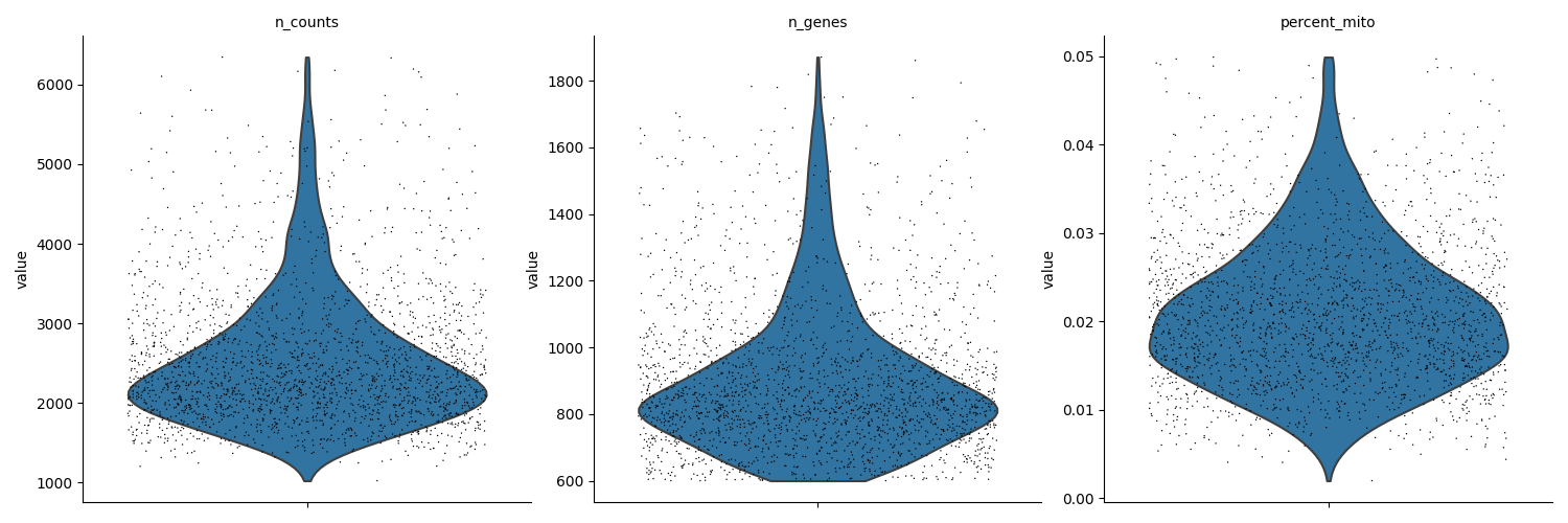
Using the chosen thresholds the data is filtered. Before and after filtering results are depicted to compare.

# visualize data before filtering
sc.pl.violin(
    adata, ["n_counts", "n_genes", "percent_mito"], multi_panel=True, jitter=0.4
)

print(
    "The AnnData object currently contains:",
    str(adata.shape[0]),
    "cells and",
    str(adata.shape[1]),
    "genes",
)
print(adata)

# perform filtering
adata = bc.pp.filter(
    adata,
    max_counts=max_UMI,
    max_genes=max_genes,
    max_mito=max_mito,
    min_genes=min_genes,
    min_counts=min_UMI,
    min_cells=min_cells,
)

# visualize data after filtering
sc.pl.violin(
    adata, ["n_counts", "n_genes", "percent_mito"], multi_panel=True, jitter=0.4
)

print(
    "The AnnData object now contains:",
    str(adata.shape[0]),
    "cells and",
    str(adata.shape[1]),
    "genes",
)
print(adata)

• 
• 

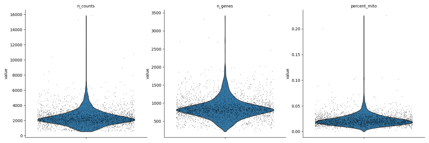
The AnnData object currently contains: 2700 cells and 32738 genes
AnnData object with n_obs × n_vars = 2700 × 32738
    obs: 'CELL', 'n_counts', 'n_genes', 'percent_mito'
    var: 'ENSEMBL', 'SYMBOL'
The AnnData object now contains: 2279 cells and 14702 genes
AnnData object with n_obs × n_vars = 2279 × 14702
    obs: 'CELL', 'n_counts', 'n_genes', 'percent_mito'
    var: 'ENSEMBL', 'SYMBOL', 'n_cells'