cluster generation

This example demonstrates how to perform highly variable gene selection, PCA, nearest neighbor calculation, and clustering.

import besca as bc
import scanpy as sc
import pytest

# pytest.skip('Test is only for here as example and should not be executed')
# import example dataset that has previously been filtered
adata = bc.datasets.pbmc3k_filtered()
## We get the raw matrix containing all the initial genes, keeping the filtering on the cells
adata = bc.get_raw(adata)

highly variable gene selection

select highly variable genes (considers correction for gene expression level)

# define thresholds for highly variable genes
variable_genes_min_mean = 0.01
variable_genes_max_mean = 5
variable_genes_min_disp = 0.4

# identify genes with variable expression
filter_result = sc.pp.filter_genes_dispersion(
    adata.X,
    min_mean=variable_genes_min_mean,
    max_mean=variable_genes_max_mean,
    min_disp=variable_genes_min_disp,
)
sc.pl.filter_genes_dispersion(filter_result)
nbr_variable_genes = sum(filter_result.gene_subset)
print("number of variable genes selected ", nbr_variable_genes)

# perform the actual filtering
adata = adata[:, filter_result.gene_subset]

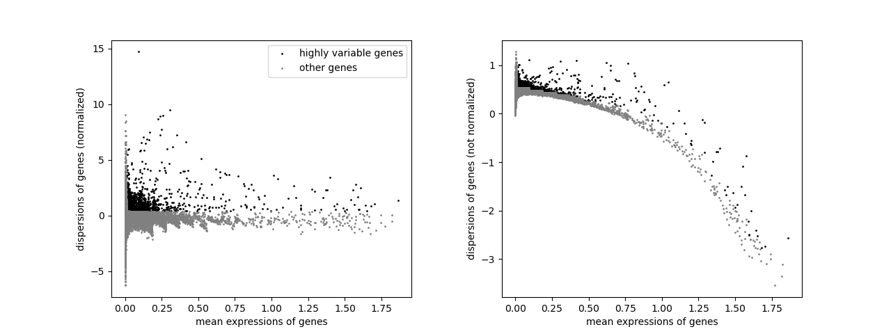
number of variable genes selected  1897

set random seed

To get reproducible results you need to define a random seed for all of the stochastic processes, such as e.g. PCA, neighbors, etc.

# set random seed
random_seed = 0

PCA

# log transform our data (is easier to work with numbers like this)
sc.pp.log1p(adata)

# Scale data to unit variance and zero mean, and cut-off at max value 10
sc.pp.scale(adata, max_value=10)

# calculate 50 principle components of the dataset
sc.tl.pca(adata, random_state=random_seed, svd_solver="arpack")

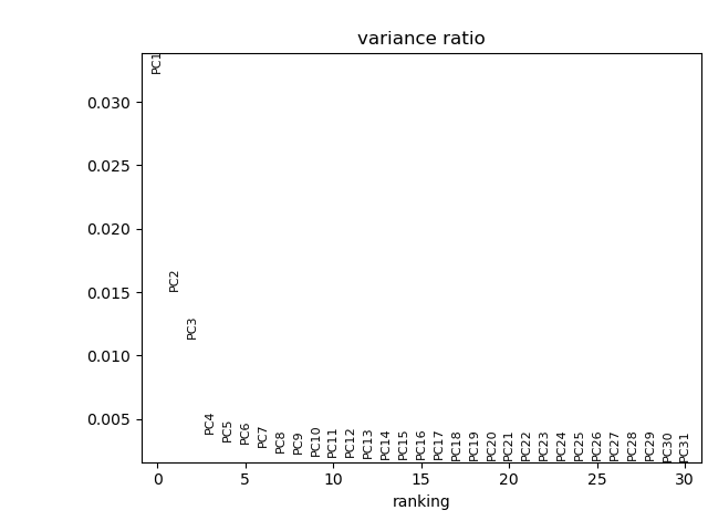
# visualize the amount of variance explained by each PC
sc.pl.pca_variance_ratio(adata)

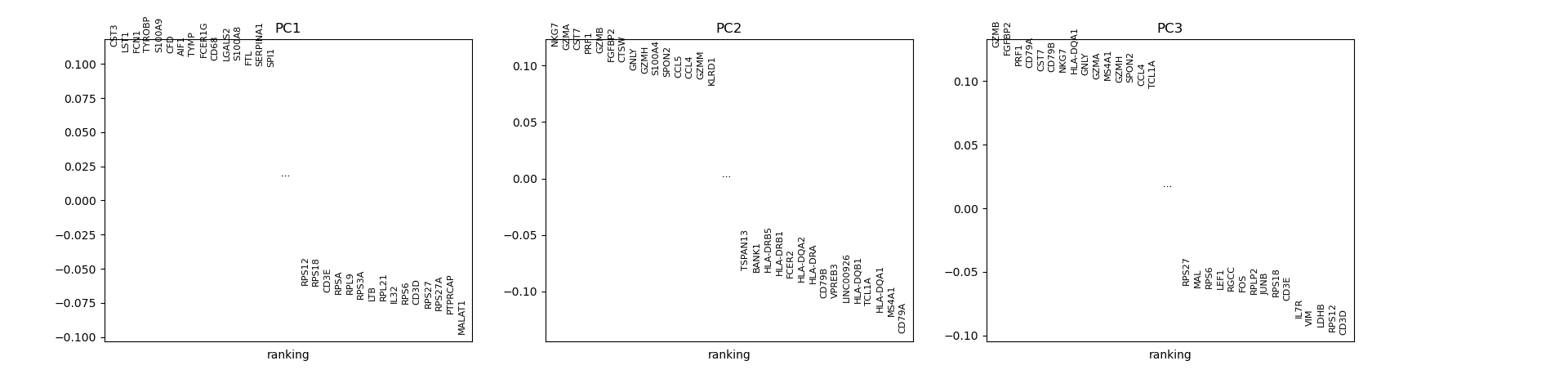
# visualize the loadings onto the first 3 PCs
sc.pl.pca_loadings(adata)

• 
• 

nearest neighbors

sc.pp.neighbors(adata, n_neighbors=15, random_state=random_seed, n_pcs=50)

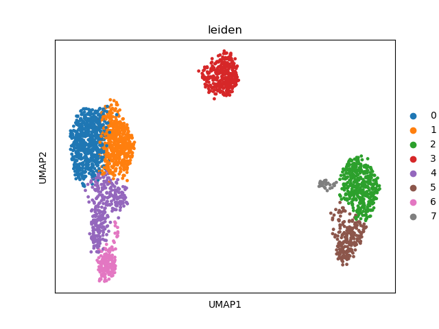
leiden clustering

sc.tl.leiden(adata, random_state=random_seed)

UMAP and t-SNE generation

# calculate UMAP
sc.tl.umap(adata, random_state=random_seed)

# calculate t-SNE
sc.tl.tsne(adata, random_state=random_seed)

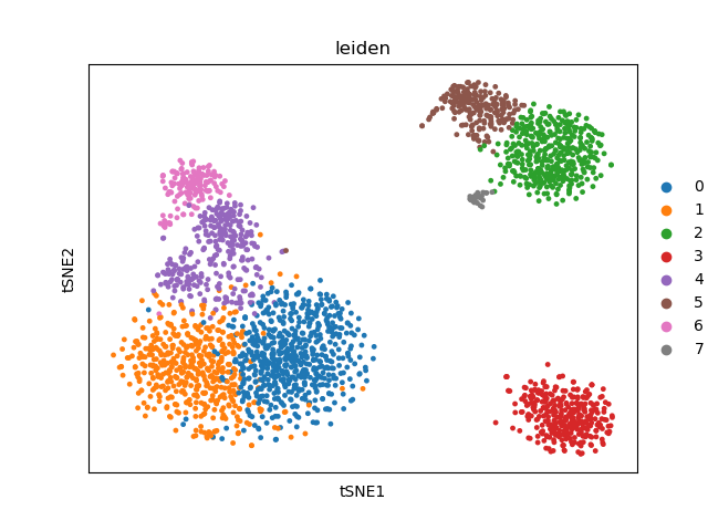
visualize the results

sc.pl.umap(adata, color=["leiden"])
sc.pl.tsne(adata, color=["leiden"])

• 
•