notebook 2 - celltype annotation and beyond
This notebook will introduce you to the process of celltype annotation and give you a brief outlook of some of the analysis you can do with single-cell data in scanpy & besca.
[1]:
#import necessary python packages
import scanpy.api as sc #software suite of tools for single-cell analysis in python
import besca as bc #internal BEDA package for single cell analysis
import matplotlib.pyplot as plt
import seaborn as sns
import pandas as pd
import numpy as np
import scipy

sc.logging.print_versions() #output an overview of the software versions that are loaded
scanpy==1.4.5.1 anndata==0.7.1 umap==0.3.10 numpy==1.16.2 scipy==1.4.1 pandas==0.24.1 scikit-learn==0.22.1 statsmodels==0.11.1 python-igraph==0.7.1 louvain==0.6.1
[2]:
from IPython.display import HTML
task = "<style>div.task { background-color: #ffc299; border-color: #ff944d; border-left: 7px solid #ff944d; padding: 1em;} </style>"
HTML(task)
[2]:
[3]:
tag = "<style>div.tag { background-color: #99ccff; border-color: #1a8cff; border-left: 7px solid #1a8cff; padding: 1em;} </style>"
HTML(tag)
[3]:
[4]:
FAIR = "<style>div.fair { background-color: #d2f7ec; border-color: #d2f7ec; border-left: 7px solid #2fbc94; padding: 1em;} </style>"
HTML(FAIR)
[4]:
Dataset
Here we will reload our previously completely processed dataset.
[5]:
#adata = sc.read('/tmp/adata_pbmc_FRESH_processed.h5ad')
adata = bc.datasets.pbmc_storage_processed()
adata.obs.drop(columns=['celltype'], inplace=True)
[6]:
adata
[6]:
AnnData object with n_obs × n_vars = 27901 × 1433
    obs: 'CELL', 'CONDITION', 'experiment', 'sample_type', 'storage_condition', 'donor', 'batch', 'n_counts', 'n_genes', 'percent_mito', 'louvain'
    var: 'ENSEMBL', 'SYMBOL', 'n_cells', 'total_counts', 'frac_reads', 'mean', 'mean_log1p', 'coeffvar', 'coeffvar_log1p'
    uns: 'donor_colors', 'louvain', 'louvain_colors', 'neighbors', 'pca', 'storage_condition_colors', 'umap'
    obsm: 'X_pca', 'X_umap'
    varm: 'PCs'
Celltype annotation
manual cell annotation based on the expression of known marker genes
[7]:
#define genes (in future you will be able to access genesets from a central database GEMS)
b_cells = ['CD19', 'CD79A', 'MS4A1']
t_cells = ['CD3E', 'CD3G', 'CD3D']
t_cell_subsets = ['CD4', 'CD8A', 'CD8B']
naive_t_cell = ['SELL', 'CCR7', 'IL7R']
myeloid_cells = ['S100A8', 'S100A9', 'CST3']
monocytes = ['FCGR3A', 'FCGR3B', 'CD14'] #FCGR3A/B = CD16
dendritic_cells = ['FCER1A', 'ITGAM', 'ITGAX'] #ITGAM = CD11b #ITGAX= CD11c
NK_cells = ['NCAM1', 'NKG7', 'CD3G']
We always use the HGNC symbols of genes as the main annotation type in the AnnData object since they are the most practical to work with. In addition, the ensemble IDs of all genes is saved in adata.var according to our FAIR standard and always written out since Ensembl IDs stay very robust over time.
Based on the dataset the marker genes that are expressed may vary strongly.
[8]:
sc.settings.set_figure_params(dpi=90)
#visualize the gene expression as an overlay of the umap
#(this way you can visually identify the clusters with a high expression))
sc.pl.umap(adata, color = b_cells, color_map = 'viridis', ncols = 3)
sc.pl.umap(adata, color = t_cells, color_map = 'viridis', ncols = 3)
sc.pl.umap(adata, color = t_cell_subsets, color_map = 'viridis', ncols = 3)
sc.pl.umap(adata, color = naive_t_cell, color_map = 'viridis', ncols = 3)
sc.pl.umap(adata, color = NK_cells,  color_map = 'viridis',ncols = 3)
sc.pl.umap(adata, color = myeloid_cells,  color_map = 'viridis',ncols = 3)
sc.pl.umap(adata, color = monocytes, color_map = 'viridis', ncols = 3)
sc.pl.umap(adata, color = dendritic_cells, color_map = 'viridis', ncols = 3)
Per default scanpy plots the gene expression values saved in adata.raw (this means log1p(cp10k)). This is the reason that we can visualize all of these genes even if they are not contained in the highly variable genes.
[9]:
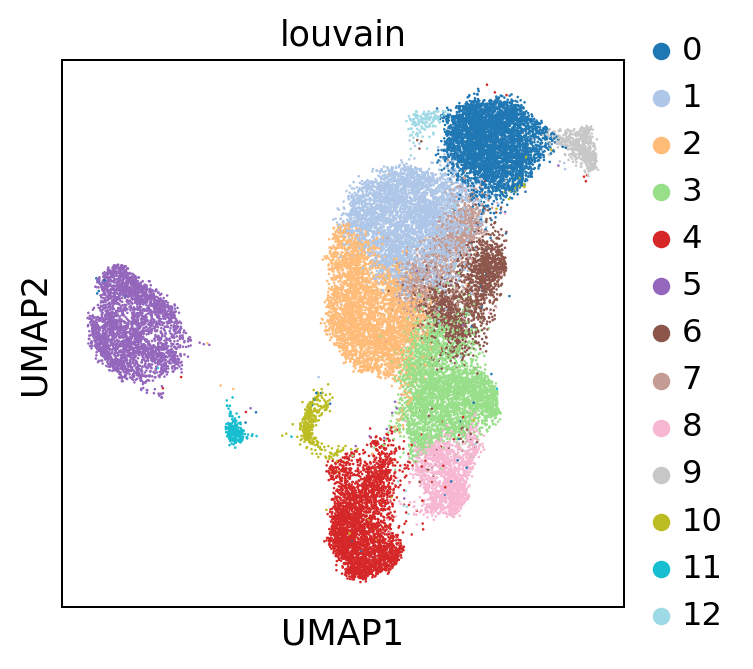
sc.pl.umap(adata, color = 'louvain', palette = 'tab20')
[10]:
#write down new cluster names (important order needs to be equivalent to above)
#will label the cell types:

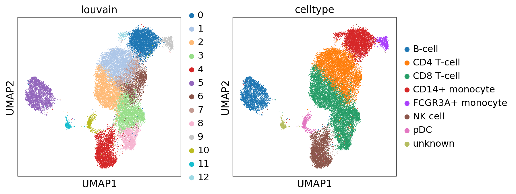
new_cluster_names = ['CD14+ monocyte', #0
                     'CD4 T-cell', #1
                     'CD8 T-cell', #2
                     'CD8 T-cell', #3
                     'NK cell', #4
                     'B-cell', #5
                     'CD4 T-cell', #6
                     'CD4 T-cell', #7
                     'CD8 T-cell', #8
                     'FCGR3A+ monocyte', #9
                     'pDC', #10
                     'unknown', #11
                     'CD14+ monocyte'] #12

bc.tl.annotate_cells_clustering(adata=adata, clustering_label='louvain', new_annotation_label='celltype', new_cluster_labels=new_cluster_names)
There are also more advanced methods of cell annotation where mixed clusters (i.e. clusters that contain more than one celltype) can be reclustered seperately and then annoated. Please refer to besca’s documentation for more information.
[11]:
sc.pl.umap(adata, color = ['louvain', 'celltype'], wspace = 0.2)
Several clusters have been combined into one celltype. Here only a very rudimentary celltype annotation was performed. Depending on the dataset and the type of analysis this can become far more complex and detailled.
write out celltype annotation
bc.st.export_celltype(adata=adata, basepath='FILEPATH_TO_FOLDER_CONTAINING_RAW_SUBFOLDER')
[12]:
bc.st.export_celltype(adata=adata, basepath='/tmp/dataset_introduction/')
mapping of cells to  celltype exported successfully to cell2labels.tsv
average.gct exported successfully to file
fract_pos.gct exported successfully to file
labelinfo.tsv successfully written out
Here we write out the celltype annotation so that we can use reload it in later analysis steps. There is a correspondng besca function for reloading the annotation.
[13]:
#save AnnData Object for comparision purposes
adata.write('/tmp/dataset_introduction/adata_pbmc_FRESH_processed_annotated.h5ad')
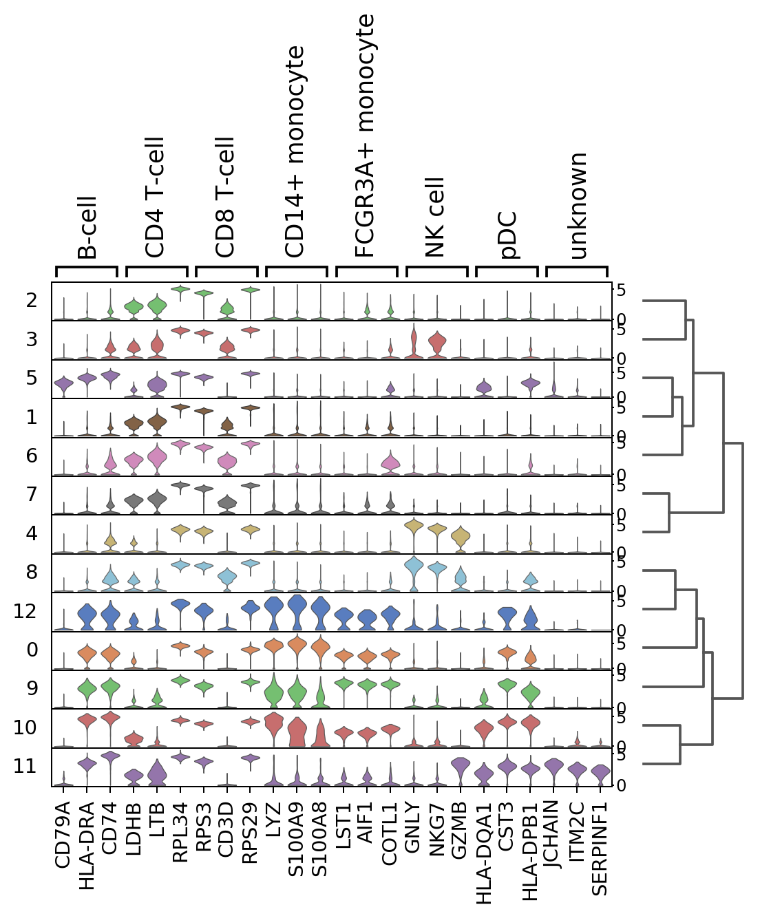
unbiased marker genes for each cluster
[14]:
#perform differential gene expression between each louvain cluster and all other cells using scanpy
sc.tl.rank_genes_groups(adata, groupby='celltype')
[15]:
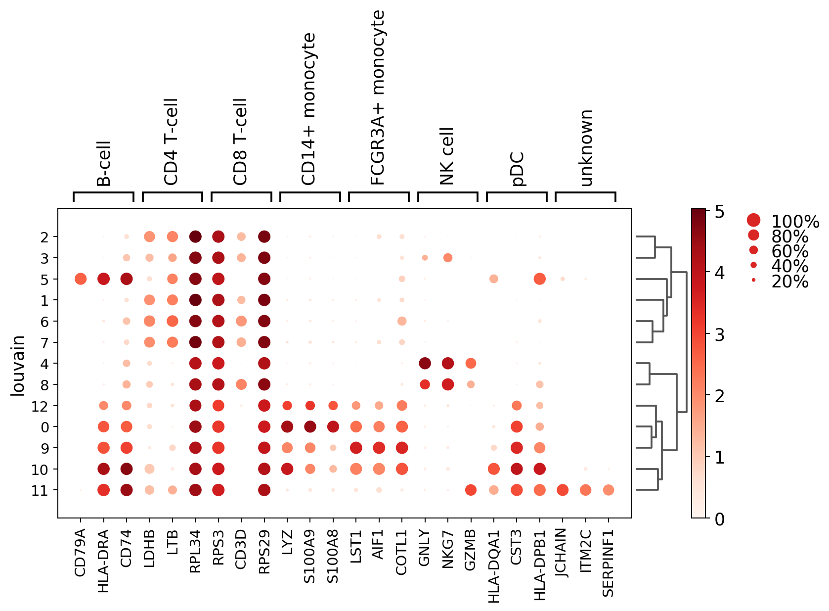
#visualize the top 3 marker genes as a dot plot
sc.pl.rank_genes_groups_dotplot(adata, n_genes=3, groupby = 'louvain')
WARNING: dendrogram data not found (using key=dendrogram_louvain). Running `sc.tl.dendrogram` with default parameters. For fine tuning it is recommended to run `sc.tl.dendrogram` independently.
WARNING: Groups are not reordered because the `groupby` categories and the `var_group_labels` are different.
categories: 0, 1, 2, etc.
var_group_labels: B-cell, CD4 T-cell, CD8 T-cell, etc.
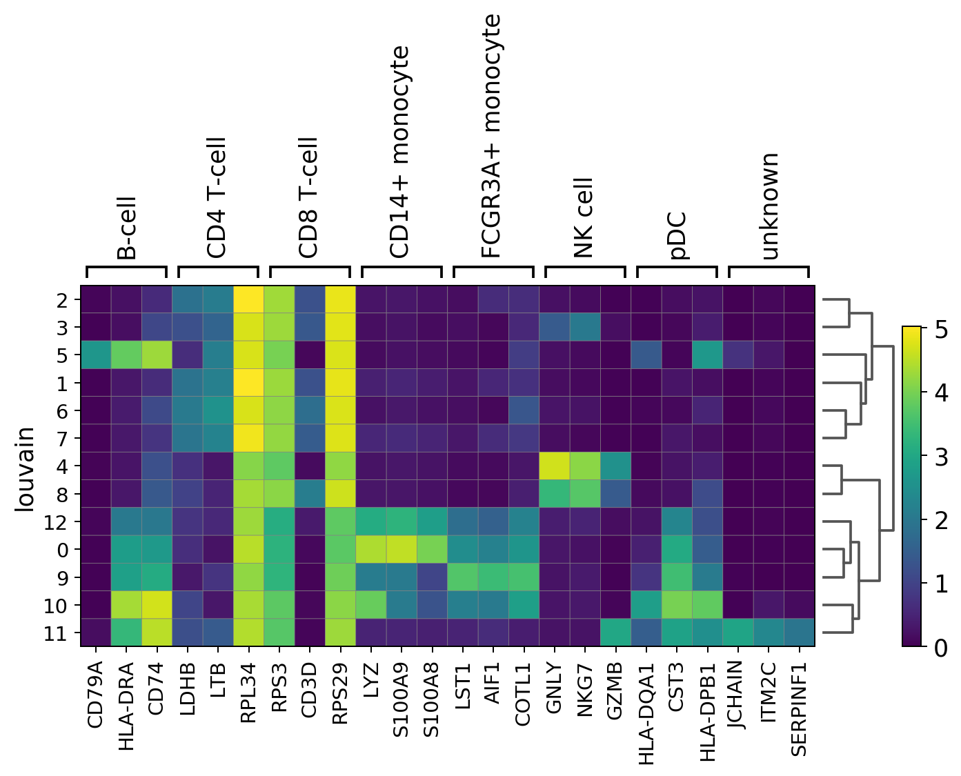
[16]:
sc.pl.rank_genes_groups_matrixplot(adata, n_genes=3, use_raw=True, groupby = 'louvain')
WARNING: Groups are not reordered because the `groupby` categories and the `var_group_labels` are different.
categories: 0, 1, 2, etc.
var_group_labels: B-cell, CD4 T-cell, CD8 T-cell, etc.
[17]:
sc.pl.rank_genes_groups_stacked_violin(adata, n_genes=3, groupby='louvain')
WARNING: Groups are not reordered because the `groupby` categories and the `var_group_labels` are different.
categories: 0, 1, 2, etc.
var_group_labels: B-cell, CD4 T-cell, CD8 T-cell, etc.
Celltype Quantification
[18]:
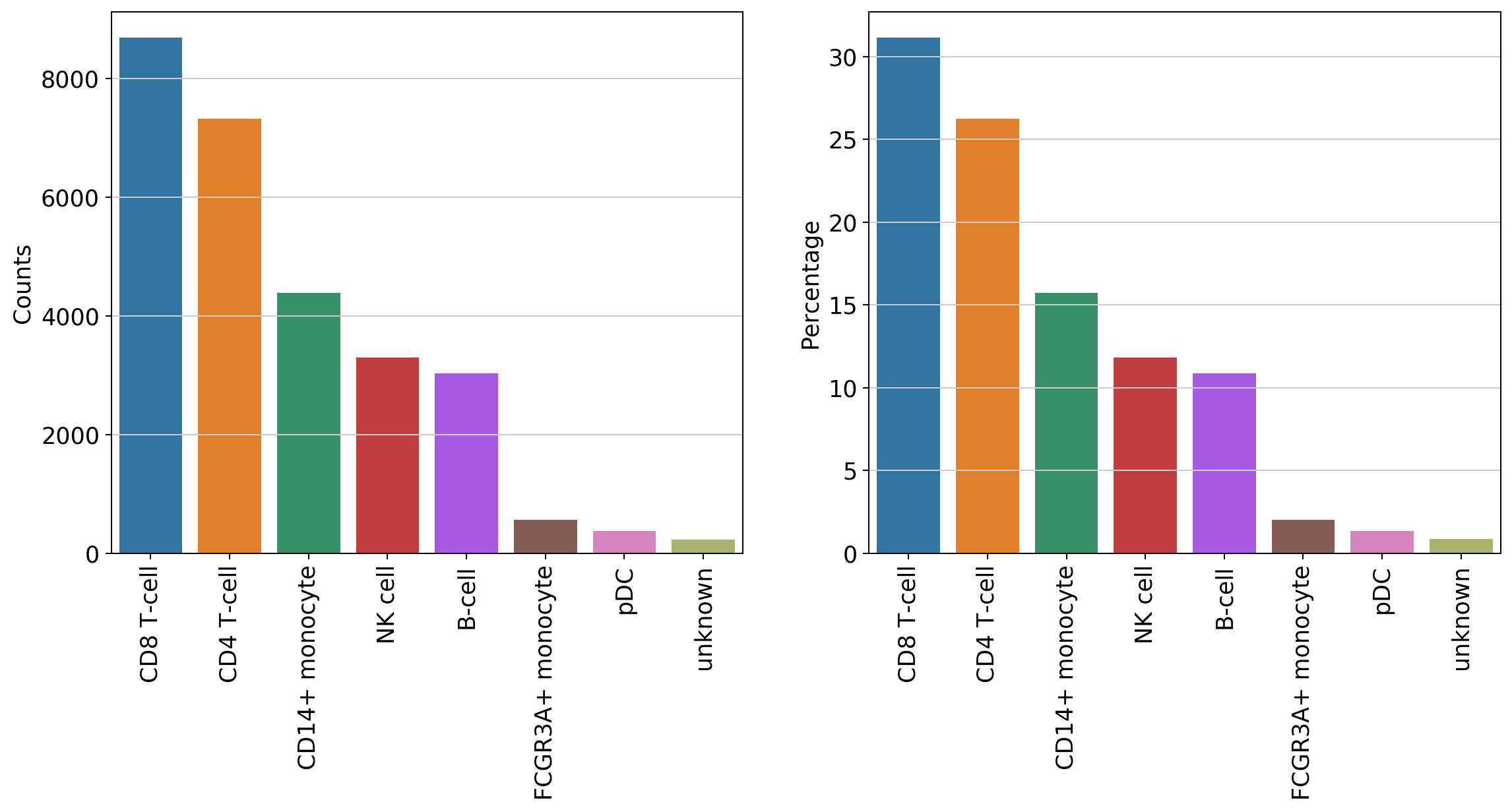
#counts per celltype
data = bc.tl.count_occurance(adata, add_percentage=True, count_variable='celltype')
display(data)
| Counts | Percentage | |
|---|---|---|
| CD8 T-cell | 8688 | 31.14 |
| CD4 T-cell | 7326 | 26.26 |
| CD14+ monocyte | 4386 | 15.72 |
| NK cell | 3295 | 11.81 |
| B-cell | 3028 | 10.85 |
| FCGR3A+ monocyte | 565 | 2.03 |
| pDC | 377 | 1.35 |
| unknown | 236 | 0.85 |
[19]:
#generate a basic bar plot of the table above
fig = plt.figure(figsize=(15,6))

#visualize distribution before logarithmization
ax1 = fig.add_subplot(1, 2, 1)
ax1 = sns.barplot(data = data, x = data.index.tolist(), y = 'Counts' )
plt.xticks(rotation=90)

#visualize distribution after logarithmization
ax2 = fig.add_subplot(1, 2, 2)
ax2 = sns.barplot(data = data, x = data.index.tolist(), y = 'Percentage' )
plt.xticks(rotation=90)
[19]:
(array([0, 1, 2, 3, 4, 5, 6, 7]), <a list of 8 Text xticklabel objects>)
[20]:
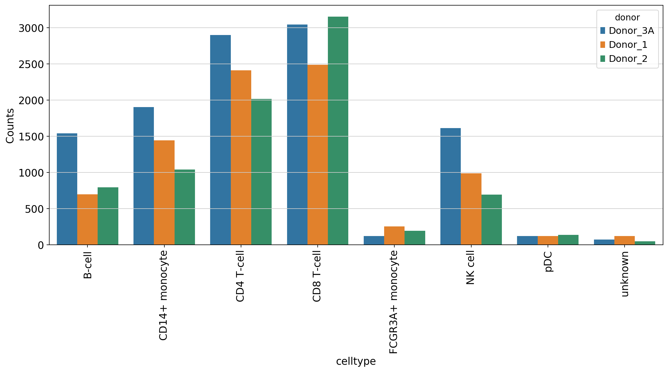
#counts on a donor level
data = bc.tl.count_occurance_subset(adata, count_variable='celltype', subset_variable='donor')
display(data)
| Donor_3A | Donor_1 | Donor_2 | |
|---|---|---|---|
| B-cell | 1539 | 697 | 792 |
| CD14+ monocyte | 1903 | 1443 | 1040 |
| CD4 T-cell | 2901 | 2410 | 2015 |
| CD8 T-cell | 3046 | 2488 | 3154 |
| FCGR3A+ monocyte | 120 | 254 | 191 |
| NK cell | 1613 | 989 | 693 |
| pDC | 119 | 121 | 137 |
| unknown | 70 | 120 | 46 |
[21]:
#make tidy for plotting
data['celltype'] = data.index.tolist()
data_plot = data.melt(value_name='Counts', id_vars='celltype', var_name='donor')

#generate a plot
fig = plt.figure(figsize=(15,6))
sns.barplot(data=data_plot, x = 'celltype', y = 'Counts', hue='donor', dodge=True)
plt.xticks(rotation=90)
[21]:
(array([0, 1, 2, 3, 4, 5, 6, 7]), <a list of 8 Text xticklabel objects>)
[22]:
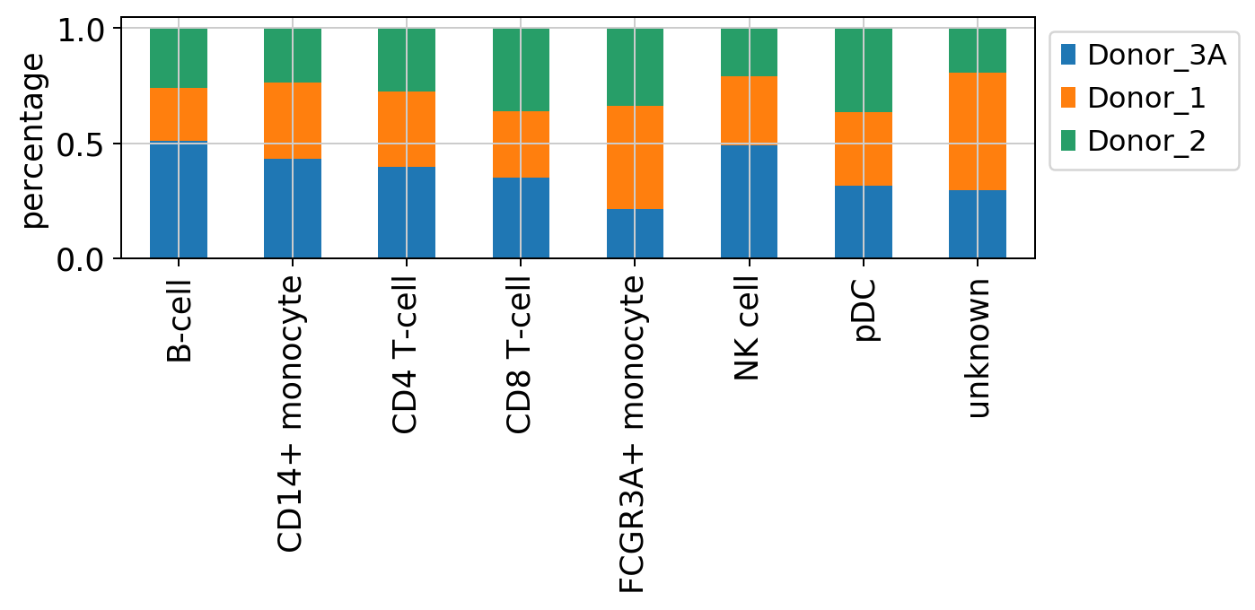
#stacked bar plot incorporated in besca
fig = bc.pl.celllabel_quant_stackedbar(adata, count_variable='celltype', subset_variable = 'donor');


