notebook 2 - celltype annotation and beyond
This notebook will introduce you to the process of celltype annotation and give you a brief outlook of some of the analysis you can do with single-cell data in scanpy & besca.
Initial visualization and hand annotation is performed here to show the possible hand-annotation and how Besca is now proposing an automated annotation process, including for mix-cluster. This procedure is done in a more straighforward manner on the same dataset in the notebook available there:
[18]:
import warnings
warnings.filterwarnings("ignore")
[19]:
#import necessary python packages
import scanpy as sc #software suite of tools for single-cell analysis in python
import besca as bc #internal BEDA package for single cell analysis
import matplotlib.pyplot as plt
import seaborn as sns
import pandas as pd
import numpy as np
import scipy

sc.logging.print_header() #output an overview of the software versions that are loaded
scanpy==1.9.1 anndata==0.8.0 umap==0.5.3 numpy==1.20.0 scipy==1.9.0 pandas==1.4.3 scikit-learn==1.1.1 statsmodels==0.13.2 python-igraph==0.9.11 pynndescent==0.5.4
[20]:
# Will only print error.
# Warning (eg genes not found) are ignored.
sc.settings.verbosity=0
[21]:
from IPython.display import HTML
task = "<style>div.task { background-color: #ffc299; border-color: #ff944d; border-left: 7px solid #ff944d; padding: 1em;} </style>"
HTML(task)
[21]:
[22]:
tag = "<style>div.tag { background-color: #99ccff; border-color: #1a8cff; border-left: 7px solid #1a8cff; padding: 1em;} </style>"
HTML(tag)
[22]:
[23]:
FAIR = "<style>div.fair { background-color: #d2f7ec; border-color: #d2f7ec; border-left: 7px solid #2fbc94; padding: 1em;} </style>"
HTML(FAIR)
[23]:
Dataset
Here we will reload our previously completely processed dataset.
[24]:
#adata = sc.read('/tmp/adata_pbmc_FRESH_processed.h5ad')
adata = bc.datasets.pbmc3k_filtered()
[25]:
adata
[25]:
AnnData object with n_obs × n_vars = 2504 × 1719
    obs: 'CELL', 'percent_mito', 'experiment', 'n_counts', 'n_genes', 'leiden'
    var: 'ENSEMBL', 'SYMBOL', 'n_cells', 'total_counts', 'frac_reads'
    uns: 'experiment_colors', 'leiden', 'leiden_colors', 'neighbors', 'pca', 'rank_genes_groups', 'umap'
    obsm: 'X_pca', 'X_umap'
    varm: 'PCs'
    obsp: 'distances', 'connectivities'
Celltype annotation
Manual cell annotation based on the expression of known marker genes
[26]:
#define genes (in future you will be able to access genesets from a central database GEMS)
b_cells = ['CD19', 'CD79A', 'MS4A1']
t_cells = ['CD3E', 'CD3G', 'CD3D']
t_cell_subsets = ['CD4', 'CD8A', 'CD8B']
naive_t_cell = ['SELL', 'CCR7', 'IL7R']
myeloid_cells = ['S100A8', 'S100A9', 'CST3']
monocytes = ['FCGR3A', 'FCGR3B', 'CD14'] #FCGR3A/B = CD16
dendritic_cells = ['FCER1A', 'ITGAM', 'ITGAX'] #ITGAM = CD11b #ITGAX= CD11c
NK_cells = ['NCAM1', 'NKG7', 'CD3G']
We always use the HGNC symbols of genes as the main annotation type in the AnnData object since they are the most practical to work with. In addition, the ensemble IDs of all genes is saved in adata.var according to our FAIR standard and always written out since Ensembl IDs stay very robust over time.
Based on the dataset the marker genes that are expressed may vary strongly.
[27]:
sc.settings.set_figure_params(dpi=90)
#visualize the gene expression as an overlay of the umap
#(this way you can visually identify the clusters with a high expression))
sc.pl.umap(adata, color = b_cells, color_map = 'viridis', ncols = 3)
sc.pl.umap(adata, color = t_cells, color_map = 'viridis', ncols = 3)
sc.pl.umap(adata, color = t_cell_subsets, color_map = 'viridis', ncols = 3)
sc.pl.umap(adata, color = naive_t_cell, color_map = 'viridis', ncols = 3)
sc.pl.umap(adata, color = NK_cells,  color_map = 'viridis',ncols = 3)
sc.pl.umap(adata, color = myeloid_cells,  color_map = 'viridis',ncols = 3)
sc.pl.umap(adata, color = monocytes, color_map = 'viridis', ncols = 3)
sc.pl.umap(adata, color = dendritic_cells, color_map = 'viridis', ncols = 3)
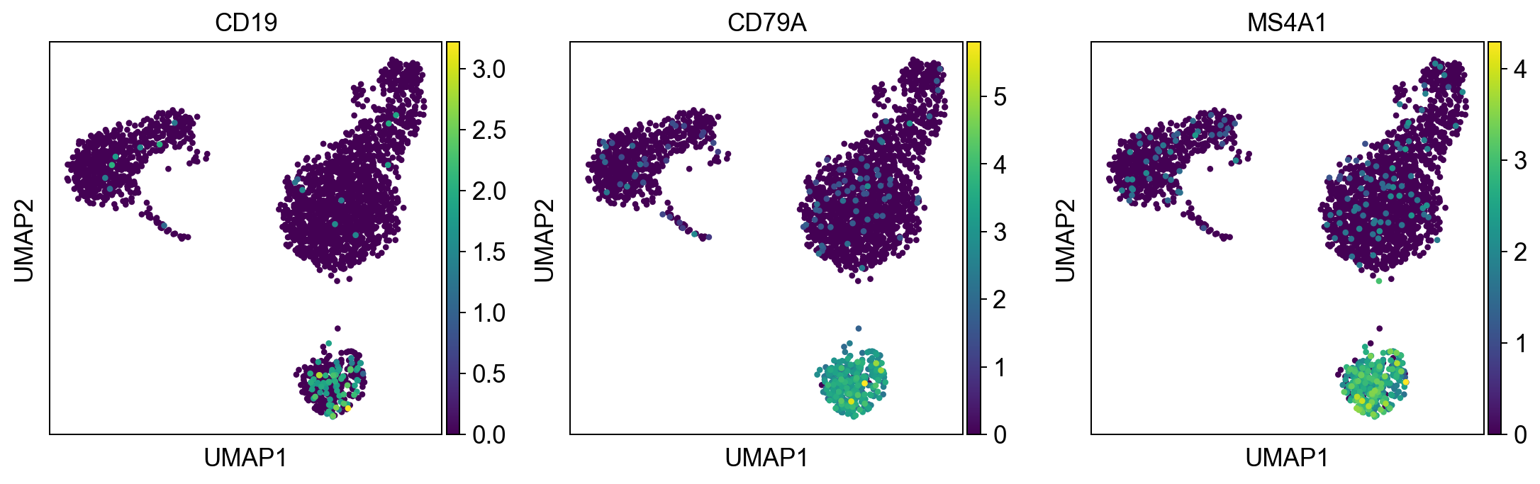
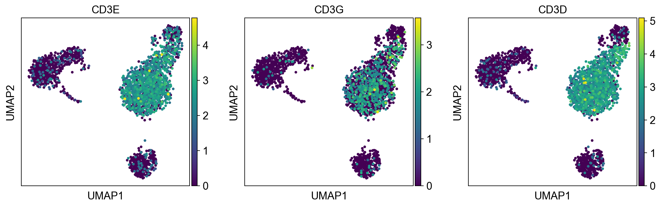
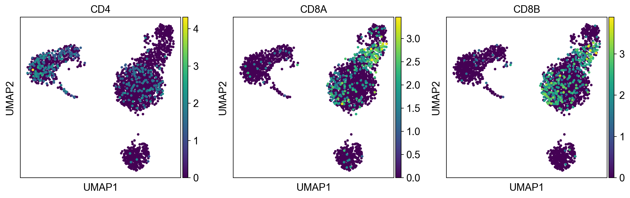
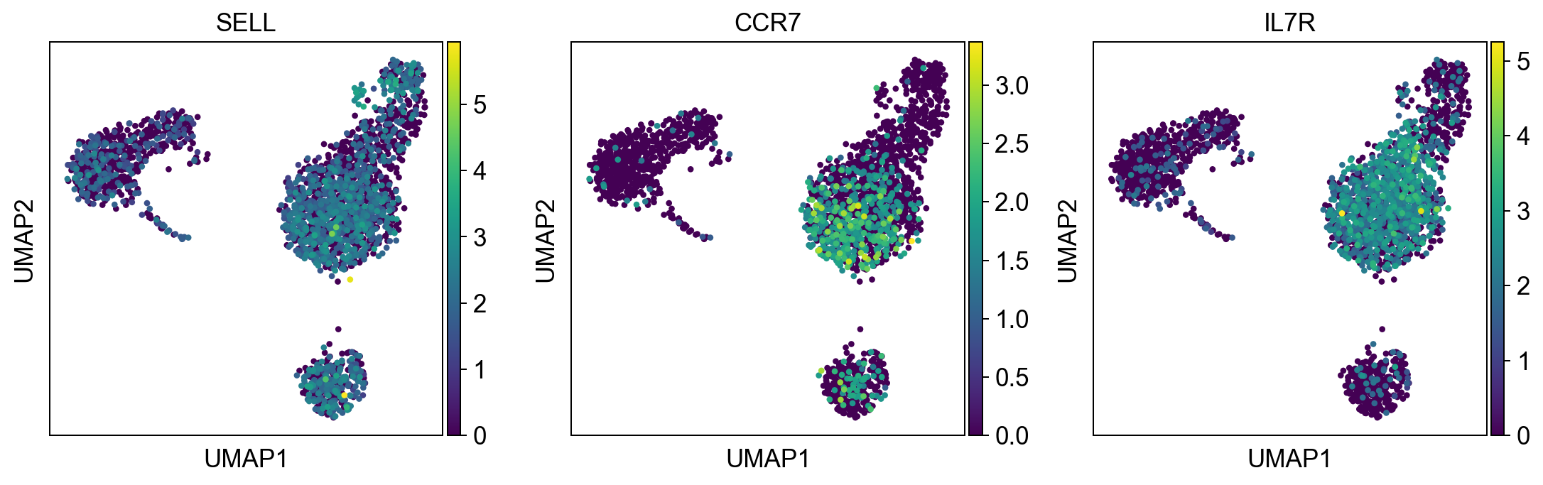
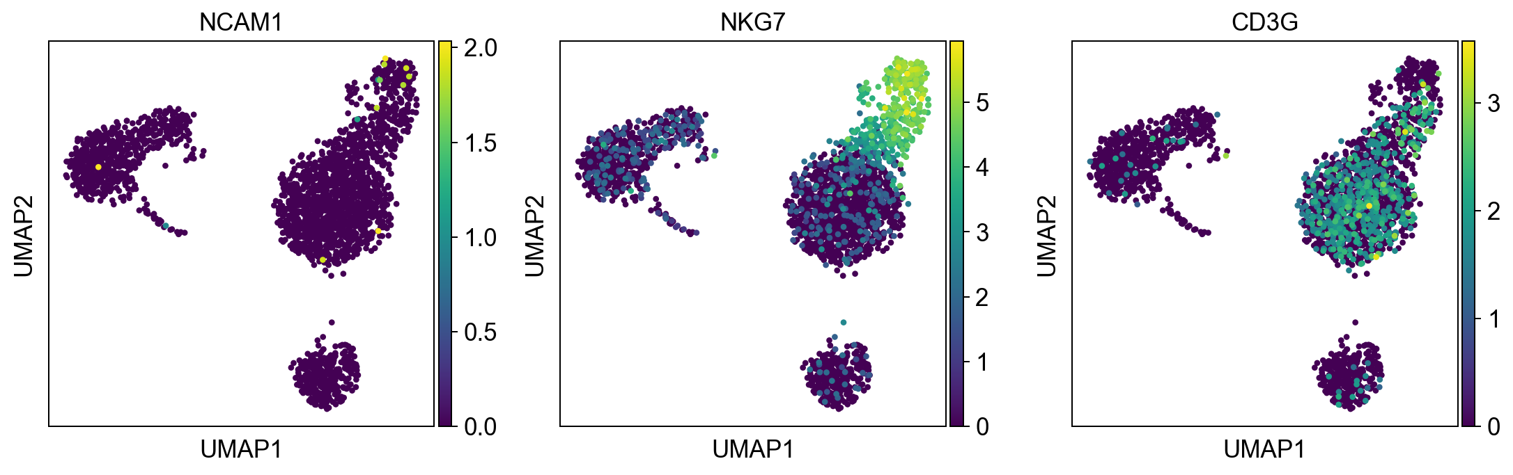
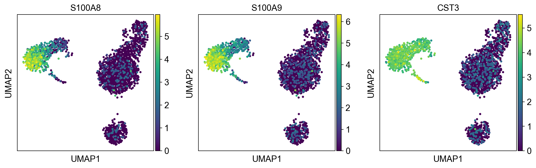
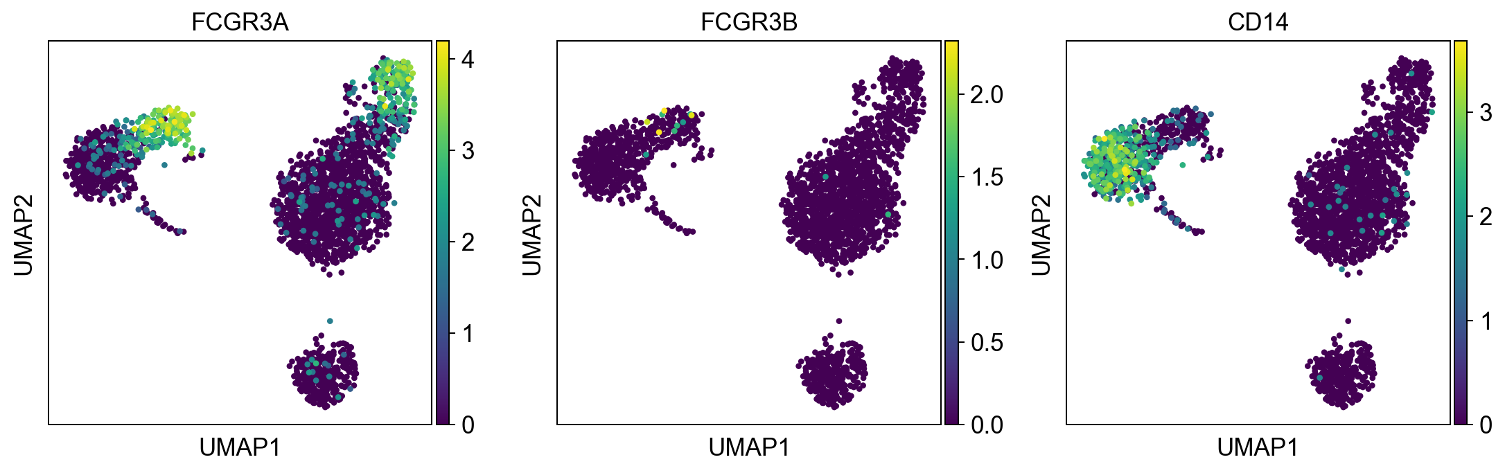
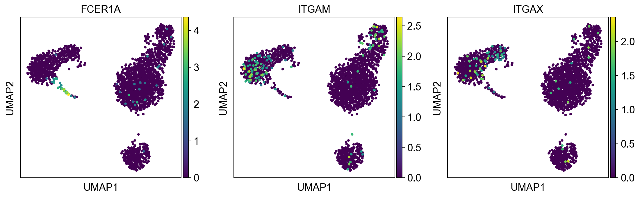
Per default scanpy plots the gene expression values saved in adata.raw (this means log1p(cp10k)). This is the reason that we can visualize all of these genes even if they are not contained in the highly variable genes.
[28]:
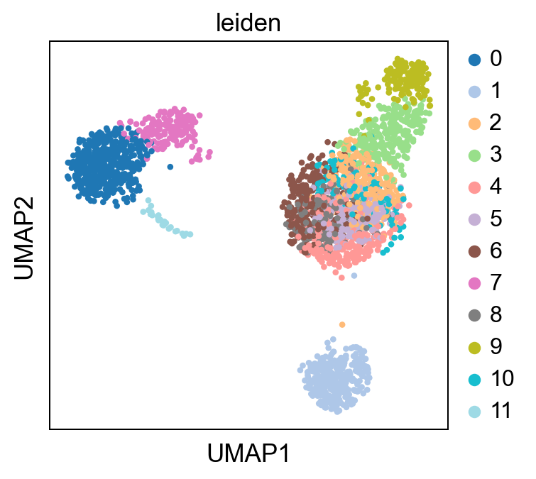
sc.pl.umap(adata, color = 'leiden', palette = 'tab20')
[29]:
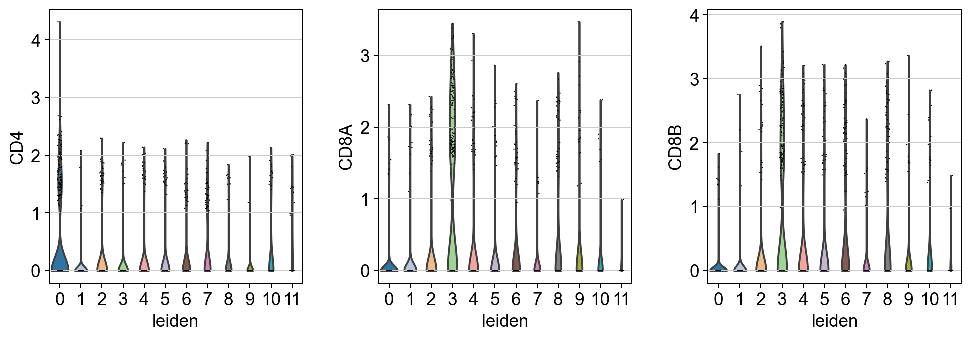
sc.pl.violin(adata, keys= t_cell_subsets, groupby= 'leiden', scale = 'count' )
[30]:
#write down new cluster names (important order needs to be equivalent to above)
#will label the cell types:

new_cluster_names = ['CD14+ monocyte', #0
                     'B-cell', #1
                     'Mix T-cell', #2
                     'CD8 T-cell', #3
                     'Mix T-cell', #4
                     'Mix T-cell', #5
                     'CD8 T-cell', #6
                     'FCGR3A+ monocyte', #7
                     'CD8 T-cell', #8
                     'NK cells', #9
                     'Mix T-cell', #10
                     'pDC'] #1

bc.tl.annotate_cells_clustering(adata=adata, clustering_label='leiden', new_annotation_label='manual_annotation', new_cluster_labels=new_cluster_names)
There are also more advanced methods of cell annotation where mixed clusters (i.e. clusters that contain more than one celltype) can be reclustered seperately and then annoated. Please refer to besca’s documentation for more information.
[31]:
sc.pl.umap(adata, color = ['leiden', 'manual_annotation'], wspace = 0.2)
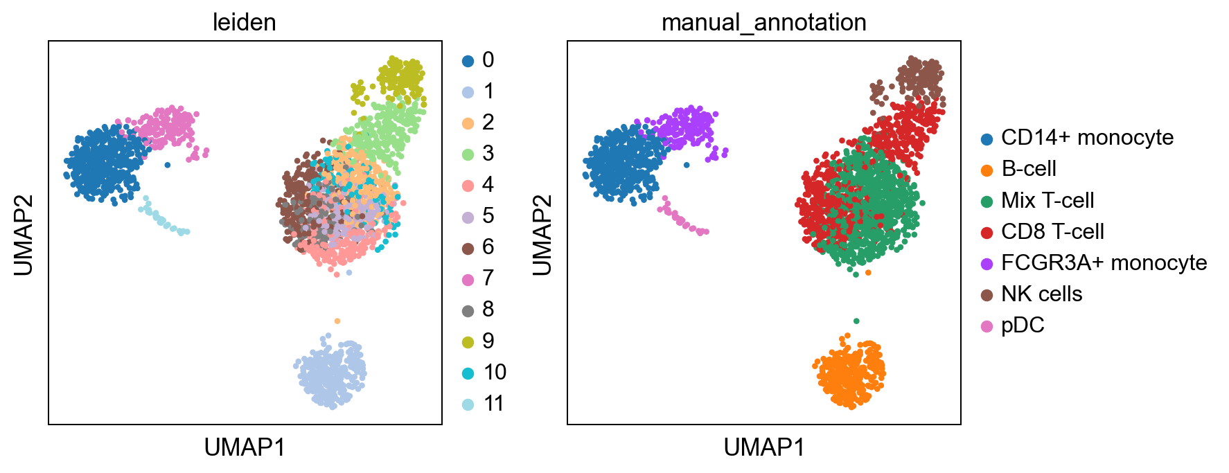
Several clusters have been combined into one celltype. Here only a very rudimentary celltype annotation was performed. Depending on the dataset and the type of analysis this can become far more complex and detailled.
We propose to use a an automated annotation methods to decipher the cluster in an un-bias way
Coffee
Tea
Milk
This steps requires to expore initial labelling. This steps within besca will export:
+ frac_pos, computing for each gene and cluster the fraction of cells that show a gene expression.
+ average.gct, computing for each gene the average expression per cluster
write out required annotation
bc.export.labeling(adata=adata, outpath=FILEPATH_TO_FOLDER, column = 'leiden')
[32]:
bc.export.write_labeling_to_files(adata=adata, outpath='dataset_export/', column = 'leiden')
mapping of cells to  leiden exported successfully to cell2labels.tsv
average.gct exported successfully to file
fract_pos.gct exported successfully to file
Hierarchical signature-enrichment based approach for cell type annotation for Hematopoeitic cells
Besca offers a hierarchical signature-enrichment based approach for cell type annotation. The initial hierarchy can be visualized below
[33]:
import pkg_resources

config_file = pkg_resources.resource_filename('besca', 'datasets/genesets/CellNames_scseqCMs6_config.tsv')
plt = bc.pl.nomenclature_network(config_file)
plt.show()
Signature loading and scoring
We load signature directly importing a gmt file. In case of connection to a GemS database, it is possible to use the GeMs signature loader.
[34]:
sigconfig,levsk=bc.tl.sig.read_annotconfig(config_file)
[35]:
gmt_file_anno = pkg_resources.resource_filename('besca', 'datasets/genesets/CellNames_scseqCMs6_sigs.gmt')


mymarkers = bc.tl.sig.read_GMT_sign(gmt_file_anno,directed=False)
mymarkers = bc.tl.sig.filter_siggenes(adata, mymarkers)


bc.tl.sig.combined_signature_score(adata, gmt_file_anno, verbose=False)
#
[36]:
sc.settings.set_figure_params(dpi=50)
scores = [x for x in adata.obs.columns if 'scanpy' in x]
sc.pl.umap(adata, color= scores, color_map = 'viridis')
Signature can be observed in detailled to assess manually the cell types to which assign the different clusters. However Besca offers to use a signature-based hierarchical annotation to build on know relations (see network above). This annotation is based on the mann whitney scoring of the positive fraction of cell and signatures provided. Additionally, this signature-based annotation procedures will then use a consistent labelling of the dataset and cell-types, facilitating cross-study comparisons in the futur.
[37]:
mymarkers['Ubi'] = ['B2M','ACTB', 'GAPDH'] ### used for cutoff adjustment to individual dataset, can be modified

f=pd.read_csv("dataset_export/fract_pos.gct",sep="\t",skiprows=2)
df=bc.tl.sig.score_mw(f,mymarkers)

myc=np.median(df.loc['Ubi',:]*0.5) ### Set a cutoff based on Ubi and scale with values from config file
One can observe the resulting log10(pvalues) obtained
[38]:
df.iloc[0:3,0:7]
[38]:
| 2 | 11 | 10 | 5 | 3 | 7 | 6 | |
|---|---|---|---|---|---|---|---|
| Bcell | 0.648278 | 2.492097 | 0.34176 | 2.251536 | 1.089847 | 0.893858 | 3.92304 |
| Fibroblast | 1.192303 | 2.057905 | 0.205498 | 2.632188 | 1.419356 | 1.432105 | 1.132777 |
| Endothelial | 0.920688 | 1.62331 | 1.262809 | 1.029862 | 0.966018 | 2.927318 | 2.748618 |
[39]:
#Cluster attribution based on cutoff
df=df.drop('Ubi')
sigscores={}
for mysig in list(df.index):
    sigscores[mysig]=bc.tl.sig.getset(df,mysig,sigconfig.loc[mysig,'Cutoff']*myc)
[40]:
sigconfig.loc["CD8Tcell","Cutoff"]=1.2
# RECOMPUTING SIG SCORE WITH NEW CUTOFF
sigscores={}
for mysig in list(df.index):
    sigscores[mysig]=bc.tl.sig.getset(df,mysig,sigconfig.loc[mysig,'Cutoff']*myc)


cnames=bc.tl.sig.make_anno(df,sigscores,sigconfig,levsk)
cnames
[40]:
| celltype0 | celltype1 | celltype2 | celltype3 | |
|---|---|---|---|---|
| 2 | Hematopoietic | Tcell | CD4Tcell | NaiCD4Tcell |
| 11 | Hematopoietic | pDC | pDC | pDC |
| 10 | Hematopoietic | Tcell | CD4Tcell | NaiCD4Tcell |
| 5 | Hematopoietic | Tcell | CD4Tcell | NaiCD4Tcell |
| 3 | Hematopoietic | Tcell | CD8Tcell | CytotoxCD8Tcell |
| 7 | Hematopoietic | Myeloid | Monocyte | NClassMonocyte |
| 6 | Hematopoietic | Tcell | CD8Tcell | NaiCD8Tcell |
| 8 | Hematopoietic | Tcell | CD8Tcell | NaiCD8Tcell |
| 4 | Hematopoietic | Tcell | CD4Tcell | NaiCD4Tcell |
| 9 | Hematopoietic | NKcell | CD56dimNK | CD56dimNK |
| 1 | Hematopoietic | Blymphocyte | Bcell | NaiBcell |
| 0 | Hematopoietic | Myeloid | Monocyte | ClassMonocyte |
[41]:
label_files = pkg_resources.resource_filename('besca', '/datasets/nomenclature/CellTypes_v1.tsv')

cnamesDBlabel = bc.tl.sig.obtain_dblabel( label_files, cnames )
cnamesDBlabel
[41]:
| celltype0 | celltype1 | celltype2 | celltype3 | |
|---|---|---|---|---|
| 2 | hematopoietic cell | T cell | CD4-positive, alpha-beta T cell | naive thymus-derived CD4-positive, alpha-beta ... |
| 11 | hematopoietic cell | plasmacytoid dendritic cell | plasmacytoid dendritic cell | plasmacytoid dendritic cell |
| 10 | hematopoietic cell | T cell | CD4-positive, alpha-beta T cell | naive thymus-derived CD4-positive, alpha-beta ... |
| 5 | hematopoietic cell | T cell | CD4-positive, alpha-beta T cell | naive thymus-derived CD4-positive, alpha-beta ... |
| 3 | hematopoietic cell | T cell | CD8-positive, alpha-beta T cell | CD8-positive, alpha-beta cytotoxic T cell |
| 7 | hematopoietic cell | myeloid leukocyte | monocyte | non-classical monocyte |
| 6 | hematopoietic cell | T cell | CD8-positive, alpha-beta T cell | naive thymus-derived CD8-positive, alpha-beta ... |
| 8 | hematopoietic cell | T cell | CD8-positive, alpha-beta T cell | naive thymus-derived CD8-positive, alpha-beta ... |
| 4 | hematopoietic cell | T cell | CD4-positive, alpha-beta T cell | naive thymus-derived CD4-positive, alpha-beta ... |
| 9 | hematopoietic cell | natural killer cell | cytotoxic CD56-dim natural killer cell | cytotoxic CD56-dim natural killer cell |
| 1 | hematopoietic cell | lymphocyte of B lineage | B cell | naive B cell |
| 0 | hematopoietic cell | myeloid leukocyte | monocyte | classical monocyte |
[42]:
adata.obs['celltype0']=bc.tl.sig.add_anno(adata,cnamesDBlabel,'celltype0','leiden')
adata.obs['celltype1']=bc.tl.sig.add_anno(adata,cnamesDBlabel,'celltype1','leiden')
adata.obs['celltype2']=bc.tl.sig.add_anno(adata,cnamesDBlabel,'celltype2','leiden')
adata.obs['celltype3']=bc.tl.sig.add_anno(adata,cnamesDBlabel,'celltype3','leiden')
[43]:
sc.pl.umap(adata,color=['leiden','celltype2', 'celltype1',
                        'CD8A', 'CD8B', # CD8 T cell markers
                        'CD4' ,    'GPR183', 'CMTM8' # CD4 t cell markers
                       ], ncols=2) #,'celltype3'
Here we believe some clusters of T cells are still mixed and that a more refined annotation can be done if recluster the lymphocytes. This procedure is applied below
Reclustering Lymphocytes
[44]:
adata.obs['leiden_original'] = adata.obs['leiden'].copy()
[45]:
adata_rc = bc.tl.rc.recluster ( adata, celltype_label = 'celltype1',
                               celltype= ('T cell',  'natural killer cell'), resolution=1.3)
[46]:
sc.pl.umap( adata_rc, color = ['celltype2','leiden',
                              # Some markers
                              'CD3G', 'CD8A', 'CD4', 'IL7R', 'NKG7', 'GNLY'])
Exporting the additional labelling allows to regenerate frac_pos required file for the annotation function.
[47]:
adata_rc = bc.st.additional_labeling(adata_rc, 'leiden', 'Leiden_Reclustering', 'Leiden Reclustering on Lymphocytes', 'BescaTutorial', 'dataset_export')
rank genes per label calculated using method wilcoxon.
dataset_export/labelings/Leiden_Reclustering/WilxRank.gct written out
dataset_export/labelings/Leiden_Reclustering/WilxRank.pvalues.gct written out
dataset_export/labelings/Leiden_Reclustering/WilxRank.logFC.gct written out
mapping of cells to  leiden exported successfully to cell2labels.tsv
average.gct exported successfully to file
fract_pos.gct exported successfully to file
labelinfo.tsv successfully written out
[48]:
mymarkers['Ubi'] = ['B2M','ACTB', 'GAPDH']
clusters = 'Leiden_Reclustering'
f=pd.read_csv('dataset_export' + "/labelings/"+clusters+"/fract_pos.gct",sep="\t",skiprows=2)
df=bc.tl.sig.score_mw(f,mymarkers)
myc=np.median(df.loc['Ubi',:]*0.5) ### Set a cutoff based on Ubi and scale with values from config file
[49]:
# RECOMPUTING SIG SCORE WITH NEW CUTOFF
df=df.drop('Ubi')
sigscores={}
for mysig in list(df.index):
    sigscores[mysig]=bc.tl.sig.getset(df,mysig,sigconfig.loc[mysig,'Cutoff']*myc)
    #sigscores[mysig]=bc.tl.sig.getset(df,mysig,10)
[50]:
toExclude = [x  for x in levsk[1] if not x == 'Tcell' and not x == 'NKcell']

cnames=bc.tl.sig.make_anno(df,sigscores,sigconfig,levsk,  toexclude= toExclude)

cnamesDBlabel = bc.tl.sig.obtain_dblabel(label_files, cnames )


adata_rc.obs['celltype0']=bc.tl.sig.add_anno(adata_rc,cnamesDBlabel,'celltype0','leiden')
adata_rc.obs['celltype2']=bc.tl.sig.add_anno(adata_rc,cnamesDBlabel,'celltype2','leiden')
adata_rc.obs['celltype3']=bc.tl.sig.add_anno(adata_rc,cnamesDBlabel,'celltype3','leiden')
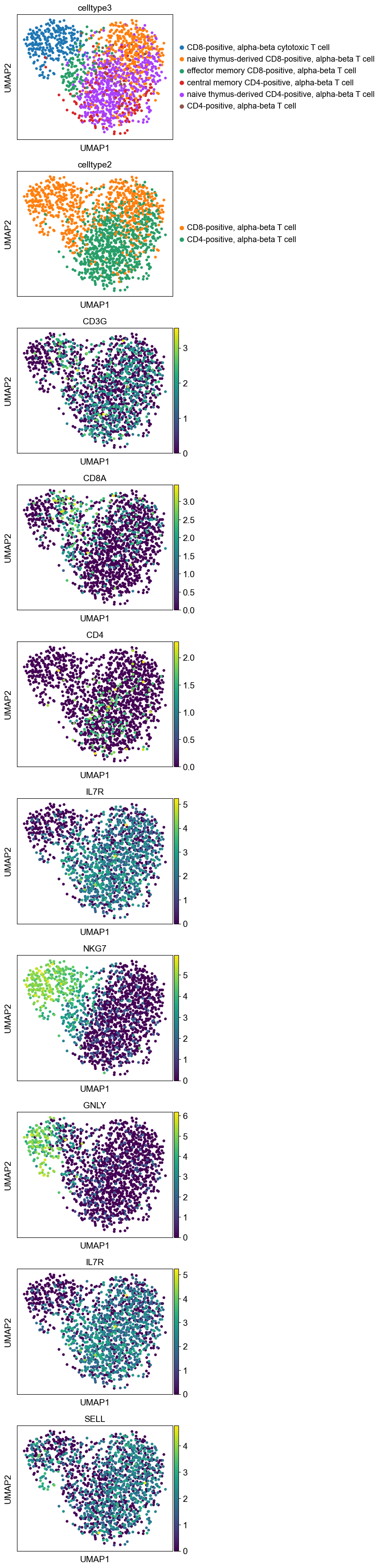
[51]:
sc.pl.umap(adata_rc,color=['celltype3', 'celltype2',
                           'CD3G', 'CD8A', 'CD4', 'IL7R', 'NKG7', 'GNLY', #, 'S100A'
                           'IL7R', 'SELL'
                          ],
           ncols=1)
[52]:
names_2 = []
names_3 = []
for i in range( cnames.shape[0]) :
    # Orderigng lexo. order
    names_2 += [cnamesDBlabel['celltype2'][str(i)]]
    names_3 += [cnamesDBlabel['celltype3'][str(i)]]
[53]:
bc.tl.rc.annotate_new_cellnames( adata, adata_rc, names = names_2, new_label='celltype2', method = 'leiden')

bc.tl.rc.annotate_new_cellnames( adata, adata_rc, names = names_3, new_label='celltype3', method = 'leiden')
[54]:
sc.pl.umap(adata,color=['celltype2',
                       'celltype3'], ncols=1, alpha= 0.9, size= 30)
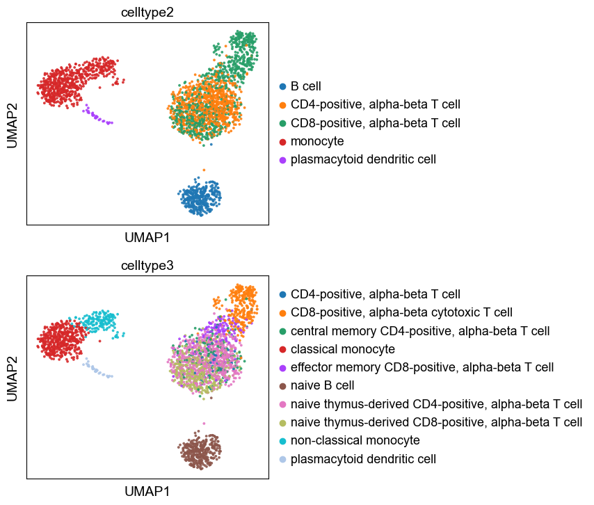
Here we write out the celltype annotation so that we can use reload it in later analysis steps. There is a corresponding besca function for reloading the annotation.
[55]:
#save AnnData Object for comparision purposes
adata.write('dataset_export/data_pbmc_processed_annotated.h5ad')
unbiased marker genes for each cluster
[56]:
#perform differential gene expression between each cluster and all other cells using scanpy
sc.tl.rank_genes_groups(adata, groupby='celltype3')
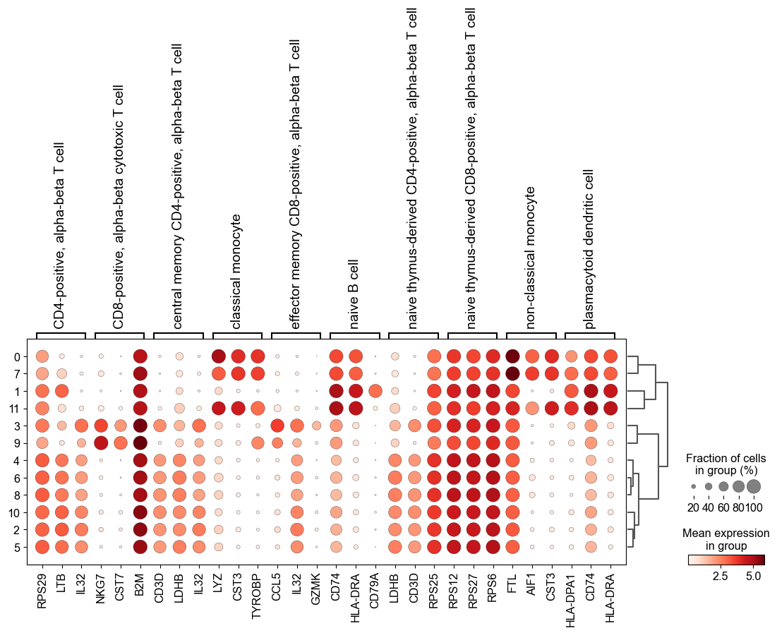
[57]:
#visualize the top 3 marker genes as a dot plot
sc.pl.rank_genes_groups_dotplot(adata, n_genes=3, groupby = 'leiden')
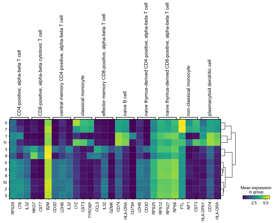
[58]:
sc.pl.rank_genes_groups_matrixplot(adata, n_genes=3, use_raw=True, groupby = 'leiden')
[59]:
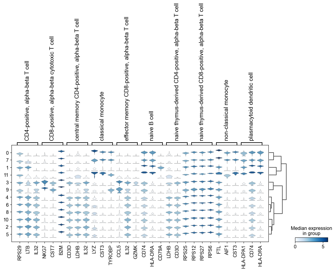
sc.pl.rank_genes_groups_stacked_violin(adata, n_genes=3, groupby='leiden')
Celltype Quantification
[60]:
#counts per celltype
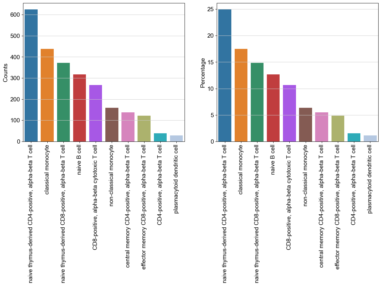
data = bc.tl.count_occurrence(adata, add_percentage=True, count_variable='celltype3')
display(data)
| Counts | Percentage | |
|---|---|---|
| naive thymus-derived CD4-positive, alpha-beta T cell | 624 | 24.92 |
| classical monocyte | 438 | 17.49 |
| naive thymus-derived CD8-positive, alpha-beta T cell | 372 | 14.86 |
| naive B cell | 317 | 12.66 |
| CD8-positive, alpha-beta cytotoxic T cell | 267 | 10.66 |
| non-classical monocyte | 159 | 6.35 |
| central memory CD4-positive, alpha-beta T cell | 138 | 5.51 |
| effector memory CD8-positive, alpha-beta T cell | 122 | 4.87 |
| CD4-positive, alpha-beta T cell | 38 | 1.52 |
| plasmacytoid dendritic cell | 29 | 1.16 |
[61]:
#generate a basic bar plot of the table above
fig = plt.figure(figsize=(15,6))

#visualize distribution before logarithmization
ax1 = fig.add_subplot(1, 2, 1)
ax1 = sns.barplot(data = data, x = data.index.tolist(), y = 'Counts' )
plt.xticks(rotation=90)

#visualize distribution after logarithmization
ax2 = fig.add_subplot(1, 2, 2)
ax2 = sns.barplot(data = data, x = data.index.tolist(), y = 'Percentage' )
plt.xticks(rotation=90)
[61]:
(array([0, 1, 2, 3, 4, 5, 6, 7, 8, 9]),
 [Text(0, 0, 'naive thymus-derived CD4-positive, alpha-beta T cell'),
  Text(1, 0, 'classical monocyte'),
  Text(2, 0, 'naive thymus-derived CD8-positive, alpha-beta T cell'),
  Text(3, 0, 'naive B cell'),
  Text(4, 0, 'CD8-positive, alpha-beta cytotoxic T cell'),
  Text(5, 0, 'non-classical monocyte'),
  Text(6, 0, 'central memory CD4-positive, alpha-beta T cell'),
  Text(7, 0, 'effector memory CD8-positive, alpha-beta T cell'),
  Text(8, 0, 'CD4-positive, alpha-beta T cell'),
  Text(9, 0, 'plasmacytoid dendritic cell')])