quality control plots

This example shows you the inbuilt quality control plots from besca.

# import libraries
import besca as bc
import matplotlib.pyplot as plt
import pytest

# pytest.skip('Test is only for here as example and should not be executed')

Before beginning any analysis it is useful to take a detailled look at your dataset to get an understanding for its characteristics.

# import data
adata = bc.datasets.pbmc3k_raw()

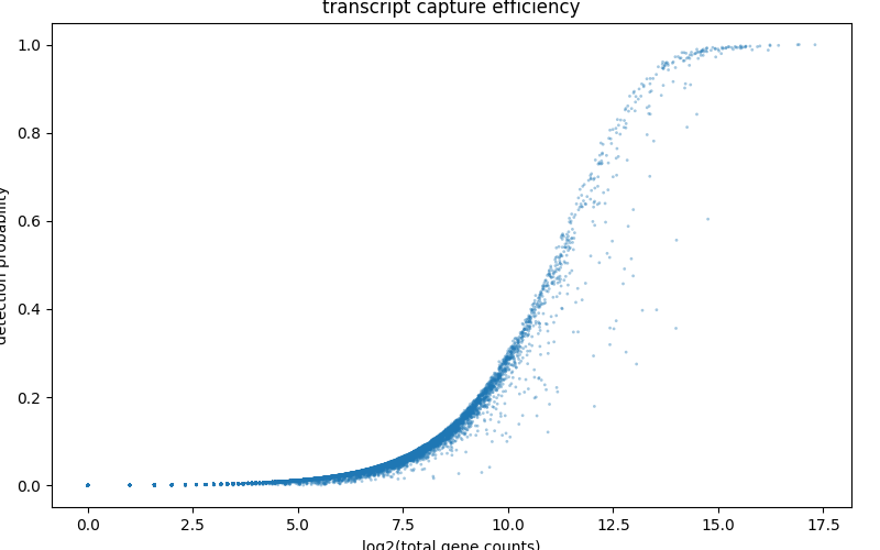
transcript capture efficiency

Plotting the transcript capture efficiency will give you an overview of the expression of genes within cells relative to the total UMI counts.

# transcript capture efficiency
fig, ax = plt.subplots(1)
fig.set_figwidth(8)
fig.set_figheight(5)
fig.tight_layout()

bc.pl.transcript_capture_efficiency(adata, ax=ax)

overview of library size unprocessed

This gives you an overview of the read distribution per cell. High quality cells will have a larger number of reads per cell and this is a parameter you can use to filter out low quality cells. The number of reads you would expect per cell is strongly dependent on the single-cell sequencing method you used.

bc.pl.librarysize_overview(adata)

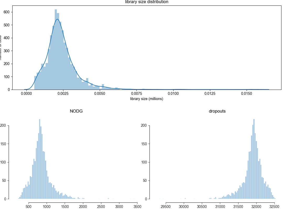
<Figure size 1100x800 with 3 Axes>

most strongly expressed transcripts

This will let you identify the genes which dominant your experiment (generally you would expect mitochondrial and ribosomal genes, in this dataset these genes have been removed beforehand).

bc.pl.top_genes_counts(adata=adata, top_n=25)

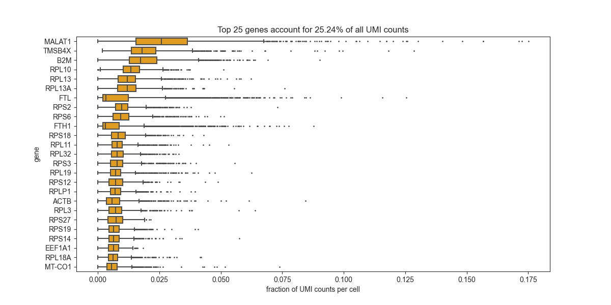
<AxesSubplot:title={'center':'Top 25 genes account for 25.24% of all UMI counts'}, xlabel='fraction of UMI counts per cell', ylabel='gene'>

visualize the processed dataset

After performing your filtering it is generally a good idea to take another look at your dataset to ensure that the filtering parameters used were reasonable.

adata = bc.datasets.pbmc3k_processed()

Please note that the displayed counts have already been scaled. You would now expect a more or less normal distribution of library size within your dataset.

bc.pl.librarysize_overview(adata)

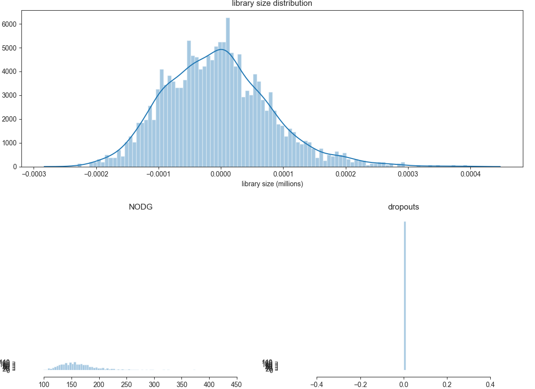
<Figure size 1100x800 with 3 Axes>