library(designit)
library(ggplot2)
library(dplyr)
#>
#> Attaching package: 'dplyr'
#> The following objects are masked from 'package:stats':
#>
#>     filter, lag
#> The following objects are masked from 'package:base':
#>
#>     intersect, setdiff, setequal, union
library(tidyr)
Plate layout with two factors
The samples
Samples of a 2-condition in-vivo experiment are to be placed on 48 well plates.
These are the conditions
# conditions to use
conditions <- data.frame(
  group = c(1, 2, 3, 4, 5),
  treatment = c(
    "vehicle", "TRT1", "TRT2",
    "TRT1", "TRT2"
  ),
  dose = c(0, 25, 25, 50, 50)
)

gt::gt(conditions)| group | treatment | dose |
|---|---|---|
| 1 | vehicle | 0 |
| 2 | TRT1 | 25 |
| 3 | TRT2 | 25 |
| 4 | TRT1 | 50 |
| 5 | TRT2 | 50 |
We will have 3 animals per groups with 4 replicates each
# sample table (2 animals per group with 3 replicates)
n_reps <- 4
n_animals <- 3
animals <- bind_rows(replicate(n_animals, conditions, simplify = FALSE),
  .id = "animal"
)
samples <- bind_rows(replicate(n_reps, animals, simplify = FALSE),
  .id = "replicate"
) |>
  mutate(
    SampleID = paste0(treatment, "_", animal, "_", replicate),
    AnimalID = paste0(treatment, "_", animal)
  ) |>
  mutate(dose = factor(dose))

samples |>
  head(10) |>
gt::gt()| replicate | animal | group | treatment | dose | SampleID | AnimalID |
|---|---|---|---|---|---|---|
| 1 | 1 | 1 | vehicle | 0 | vehicle_1_1 | vehicle_1 |
| 1 | 1 | 2 | TRT1 | 25 | TRT1_1_1 | TRT1_1 |
| 1 | 1 | 3 | TRT2 | 25 | TRT2_1_1 | TRT2_1 |
| 1 | 1 | 4 | TRT1 | 50 | TRT1_1_1 | TRT1_1 |
| 1 | 1 | 5 | TRT2 | 50 | TRT2_1_1 | TRT2_1 |
| 1 | 2 | 1 | vehicle | 0 | vehicle_2_1 | vehicle_2 |
| 1 | 2 | 2 | TRT1 | 25 | TRT1_2_1 | TRT1_2 |
| 1 | 2 | 3 | TRT2 | 25 | TRT2_2_1 | TRT2_2 |
| 1 | 2 | 4 | TRT1 | 50 | TRT1_2_1 | TRT1_2 |
| 1 | 2 | 5 | TRT2 | 50 | TRT2_2_1 | TRT2_2 |
Plate layout requirements
Corner wells of the plates should be left empty. This means on a 48 well plate we can place 44 samples. Since we have 60 samples, they will fit on 2 plates
Setting up a Batch container
Create a BatchContainer object that provides all possible locations
bc <- BatchContainer$new(
  dimensions = c("plate" = n_plates, "column" = 8, "row" = 6),
  exclude = exclude_wells
)
bc
#> Batch container with 88 locations.
#>   Dimensions: plate, column, row

bc$n_locations
#> [1] 88
bc$exclude
#> NULL
bc$get_locations() |> head()
#> # A tibble: 6 × 3
#>   plate column   row
#>   <int>  <int> <int>
#> 1     1      1     2
#> 2     1      1     3
#> 3     1      1     4
#> 4     1      1     5
#> 5     1      2     1
#> 6     1      2     2
Moving samples
Use random assignment function to place samples to plate locations
bc <- assign_random(bc, samples)

bc$get_samples()
#> # A tibble: 88 × 10
#>    plate column   row replicate animal group treatment dose  SampleID   AnimalID
#>    <int>  <int> <int> <chr>     <chr>  <dbl> <chr>     <fct> <chr>      <chr>
#>  1     1      1     2 3         3          1 vehicle   0     vehicle_3… vehicle…
#>  2     1      1     3 1         3          3 TRT2      25    TRT2_3_1   TRT2_3
#>  3     1      1     4 1         1          3 TRT2      25    TRT2_1_1   TRT2_1
#>  4     1      1     5 4         2          3 TRT2      25    TRT2_2_4   TRT2_2
#>  5     1      2     1 NA        NA        NA NA        NA    NA         NA
#>  6     1      2     2 NA        NA        NA NA        NA    NA         NA
#>  7     1      2     3 4         1          5 TRT2      50    TRT2_1_4   TRT2_1
#>  8     1      2     4 NA        NA        NA NA        NA    NA         NA
#>  9     1      2     5 NA        NA        NA NA        NA    NA         NA
#> 10     1      2     6 4         3          5 TRT2      50    TRT2_3_4   TRT2_3
#> # ℹ 78 more rows
bc$get_samples(remove_empty_locations = TRUE)
#> # A tibble: 60 × 10
#>    plate column   row replicate animal group treatment dose  SampleID   AnimalID
#>    <int>  <int> <int> <chr>     <chr>  <dbl> <chr>     <fct> <chr>      <chr>
#>  1     1      1     2 3         3          1 vehicle   0     vehicle_3… vehicle…
#>  2     1      1     3 1         3          3 TRT2      25    TRT2_3_1   TRT2_3
#>  3     1      1     4 1         1          3 TRT2      25    TRT2_1_1   TRT2_1
#>  4     1      1     5 4         2          3 TRT2      25    TRT2_2_4   TRT2_2
#>  5     1      2     3 4         1          5 TRT2      50    TRT2_1_4   TRT2_1
#>  6     1      2     6 4         3          5 TRT2      50    TRT2_3_4   TRT2_3
#>  7     1      3     1 2         3          2 TRT1      25    TRT1_3_2   TRT1_3
#>  8     1      3     2 4         2          5 TRT2      50    TRT2_2_4   TRT2_2
#>  9     1      3     3 4         3          3 TRT2      25    TRT2_3_4   TRT2_3
#> 10     1      3     4 3         3          2 TRT1      25    TRT1_3_3   TRT1_3
#> # ℹ 50 more rows
Plot of the result using the plot_plate function
plot_plate(bc,
  plate = plate, column = column, row = row,
  .color = treatment, .alpha = dose
)
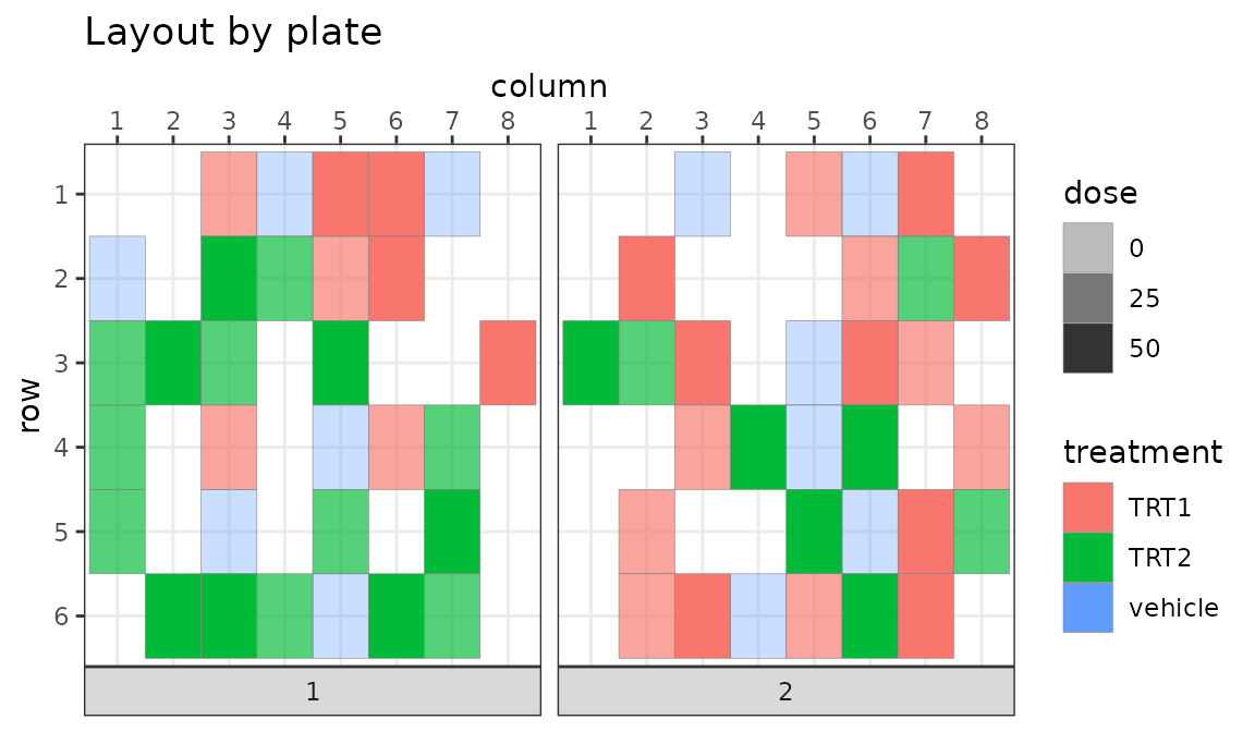
To not show empty wells, we can directly plot the sample table as
well
plot_plate(bc$get_samples(remove_empty_locations = TRUE),
  plate = plate, column = column, row = row,
  .color = treatment, .alpha = dose
)
To move individual samples or manually assigning all locations we can
use the batchContainer$move_samples() method
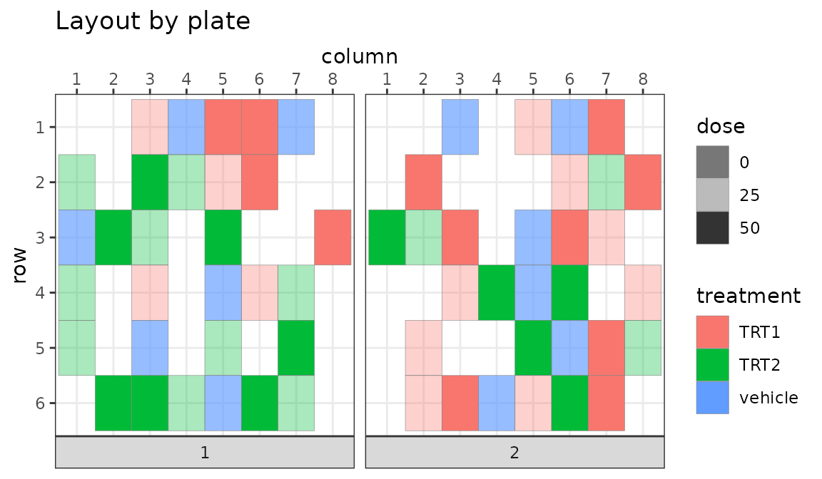
To swap two or more samples use:
Warning: This will change your BatchContainer in-place.
bc$move_samples(src = c(1L, 2L), dst = c(2L, 1L))

plot_plate(bc$get_samples(remove_empty_locations = TRUE),
  plate = plate, column = column, row = row,
  .color = treatment, .alpha = dose
)
To assign all samples in one go, use the option
location_assignment.
Warning: This will change your BatchContainer in-place.
The example below orders samples by ID and adds the empty locations afterwards
bc$move_samples(
  location_assignment = c(
    1:nrow(samples),
    rep(NA, (bc$n_locations - nrow(samples)))
  )
)

plot_plate(bc$get_samples(remove_empty_locations = TRUE, include_id = TRUE),
  plate = plate, column = column, row = row,
  .color = .sample_id
)
Run an optimization
The optimization procedure is invoked with
e.g. optimize_design. Here we use a simple shuffling
schedule: swap 10 samples for 100 times, then swap 2 samples for 400
times.
To evaluate how good a layout is, we need a scoring function.
This function will assess how well treatment and dose are balanced across the two plates.
bc <- optimize_design(bc,
  scoring = osat_score_generator(
    batch_vars = "plate",
    feature_vars = c("treatment", "dose")
  ),
  # shuffling schedule
  n_shuffle = c(rep(10, 200), rep(2, 400))
)
#> Warning in osat_score(bc, batch_vars = batch_vars, feature_vars = feature_vars,
#> : NAs in features / batch columns; they will be excluded from scoring
#> Checking variances of 1-dim. score vector.
#> ... (371.295) - OK
#> Initial score: 80
#> Achieved score: 62 at iteration 1
#> Achieved score: 44 at iteration 2
#> Achieved score: 30 at iteration 3
#> Achieved score: 26 at iteration 6
#> Achieved score: 24 at iteration 10
#> Achieved score: 16 at iteration 11
#> Achieved score: 12 at iteration 12
#> Achieved score: 6 at iteration 16
#> Achieved score: 4 at iteration 18
#> Achieved score: 2 at iteration 46
#> Achieved score: 0 at iteration 50
Development of the score can be viewed with
bc$plot_trace()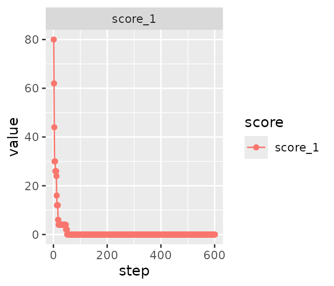
The layout after plate batching looks the following
plot_plate(bc$get_samples(remove_empty_locations = TRUE),
  plate = plate, column = column, row = row,
  .color = treatment, .alpha = dose
)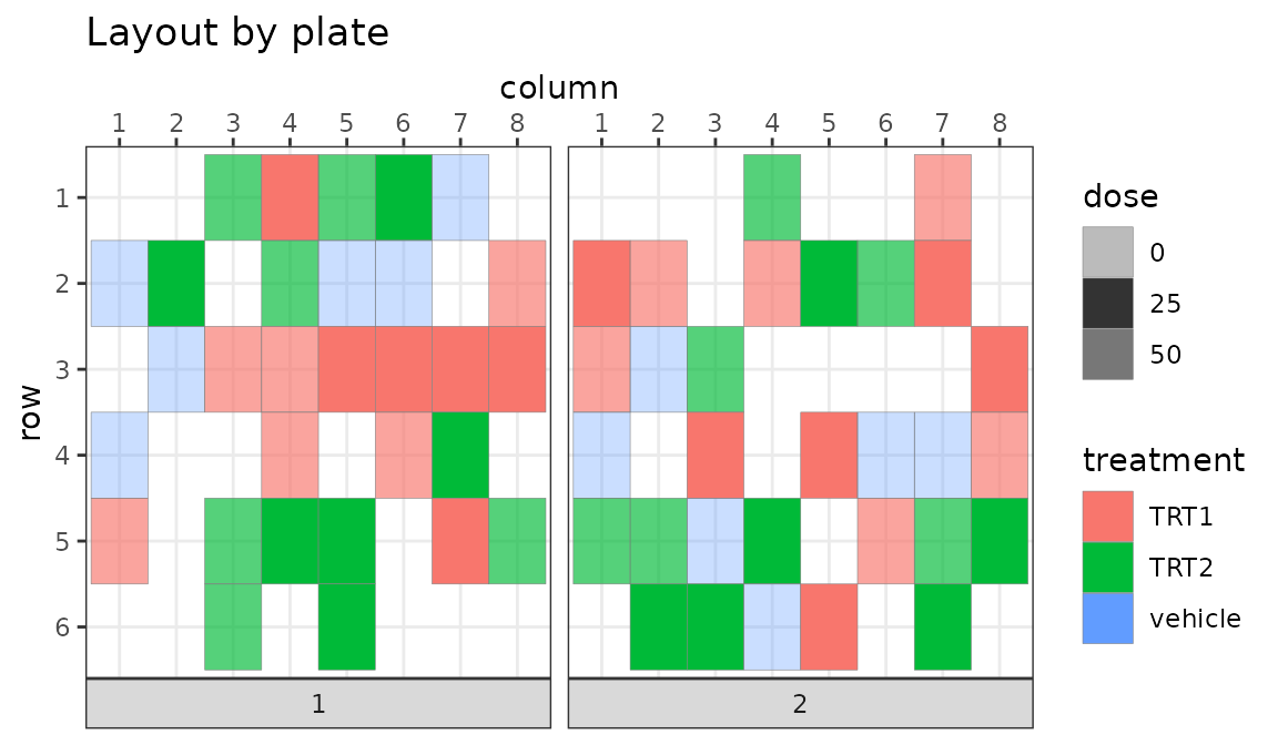
Looking at treatment, we see it’s evenly distributed across the plates
ggplot(
  bc$get_samples(remove_empty_locations = TRUE),
  aes(x = treatment, fill = treatment)
) +
  geom_bar() +
  facet_wrap(~plate)
Customizing the plate layout
To properly distinguish between empty and excluded locations one can do the following.
- Supply the BatchContainer directly
- set
add_excluded = TRUE, setrename_empty = TRUE - supply a custom color palette
- excluded wells have NA values and can be colored with
na.value
color_palette <- c(
  TRT1 = "blue", TRT2 = "purple",
  vehicle = "orange", empty = "white"
)

plot_plate(bc,
  plate = plate, column = column, row = row,
  .color = treatment, .alpha = dose,
  add_excluded = TRUE, rename_empty = TRUE
) +
  scale_fill_manual(values = color_palette, na.value = "darkgray")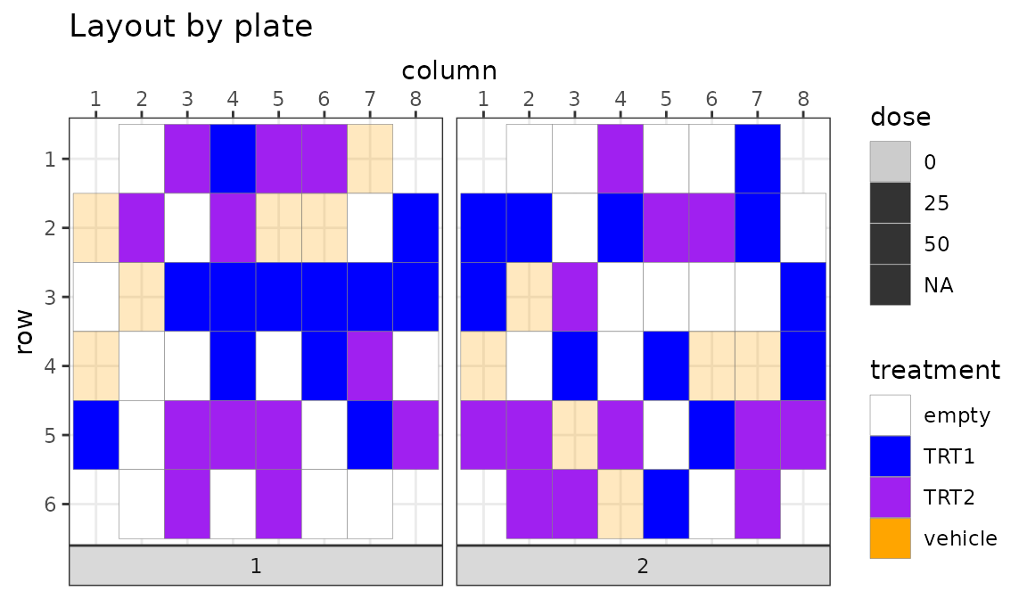
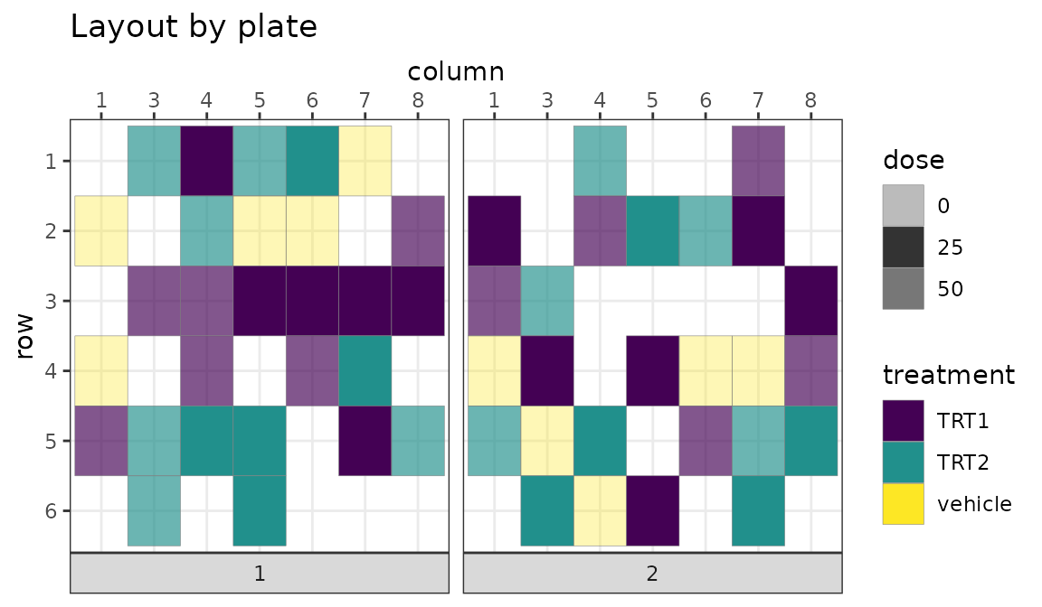
To remove all empty wells from the plot, hand the pruned sample list. to plot_plate rather than the whole BatchContainer. You can still assign your own colors.
plot_plate(bc$get_samples(remove_empty_locations = TRUE),
  plate = plate, column = column, row = row,
  .color = treatment, .alpha = dose
) +
  scale_fill_viridis_d()
Note: removing all empty and excluded wells will lead to omitting completely empty rows or columns!
plot_plate(bc$get_samples(remove_empty_locations = TRUE) |>
  filter(column != 2),
plate = plate, column = column, row = row,
.color = treatment, .alpha = dose
) +
  scale_fill_viridis_d()