In this vignette, we demonstrate how to use the OSAT score (Yan et al. (2012)).
library(designit)
library(tidyverse)
#> ── Attaching core tidyverse packages ──────────────────────── tidyverse 2.0.0 ──
#> ✔ dplyr     1.1.4     ✔ readr     2.1.5
#> ✔ forcats   1.0.0     ✔ stringr   1.5.1
#> ✔ ggplot2   3.5.0     ✔ tibble    3.2.1
#> ✔ lubridate 1.9.3     ✔ tidyr     1.3.1
#> ✔ purrr     1.0.2
#> ── Conflicts ────────────────────────────────────────── tidyverse_conflicts() ──
#> ✖ dplyr::filter() masks stats::filter()
#> ✖ dplyr::lag()    masks stats::lag()
#> ℹ Use the conflicted package (<http://conflicted.r-lib.org/>) to force all conflicts to become errors
if (!requireNamespace("OSAT")) {
  print("This vignette can only be rendered if `OSAT` package is installed.")
  knitr::knit_exit()
}
#> Loading required namespace: OSAT
Loading samples. We add two dummy columns to demonstrate how to choose batch columns of interest.
osat_data_path <- system.file("extdata", package = "OSAT")
samples <- read_tsv(file.path(osat_data_path, "samples.txt"),
  col_types = cols(SampleType = col_factor(), Race = col_factor(), AgeGrp = col_factor())
) |>
  mutate(dummy_var1 = rnorm(n()), dummy_var2 = str_c(SampleType, Race, sep = " "))
Running OSAT optimization
Here we use OSAT to optimize setup.
gs <- OSAT::setup.sample(samples, optimal = c("SampleType", "Race", "AgeGrp"))

gc <- OSAT::setup.container(OSAT::IlluminaBeadChip96Plate, 7, batch = "plates")

set.seed(1234)

bench::system_time(
  g_setup <- OSAT::create.optimized.setup(sample = gs, container = gc, nSim = params$iterations)
)
#> Warning in OSAT::create.optimized.setup(sample = gs, container = gc, nSim =
#> params$iterations): Using default optimization method: optimal.shuffle
#> process    real
#>   957ms   957ms

OSAT::QC(g_setup)
#>
#> Test independence between "plates" and sample variables
#>
#> Pearson's Chi-squared test
#>          Var X-squared df   p.value
#> 1 SampleType 0.4938509  6 0.9979125
#> 2       Race 0.7424849  6 0.9935279
#> 3     AgeGrp 1.8472070 24 1.0000000
#> 
Saving starting point of optimization
set.seed(1234)

g_setup_start <- OSAT::create.optimized.setup(sample = gs, container = gc, nSim = 1) |>
  OSAT::get.experiment.setup()
#> Warning in OSAT::create.optimized.setup(sample = gs, container = gc, nSim = 1):
#> Using default optimization method: optimal.shuffle
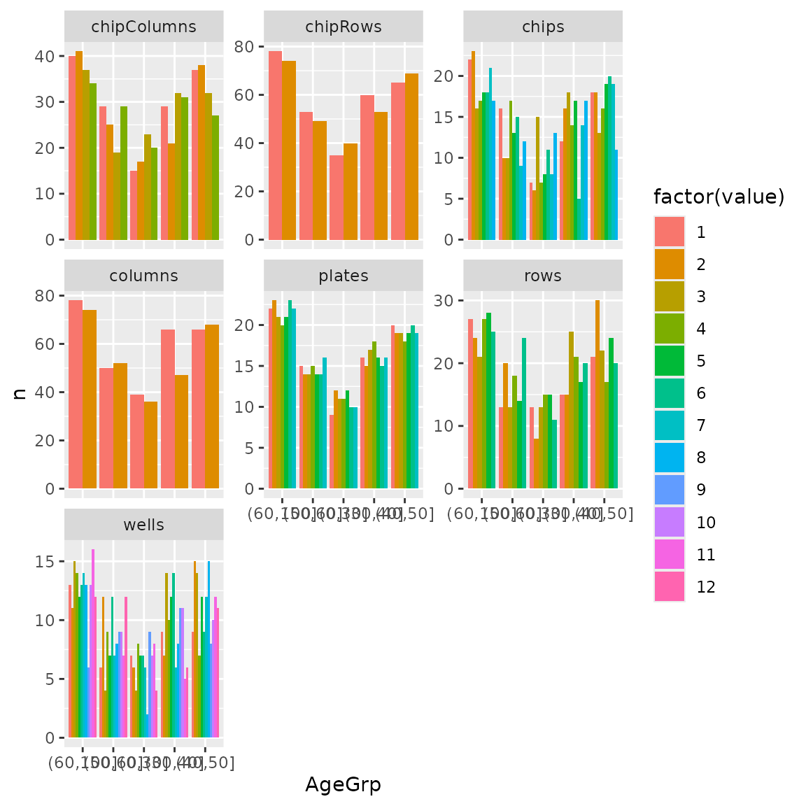
Visualize various batch factors. OSAT score is optimized only for
plates in this case.
OSAT::get.experiment.setup(g_setup) |>
  select(AgeGrp, plates, chipRows, chipColumns, chips, rows, columns, wells) |>
  pivot_longer(-AgeGrp) |>
  count(AgeGrp, value, name) |>
  ggplot(aes(AgeGrp, n, fill = factor(value))) +
  geom_col(position = "dodge") +
  facet_wrap(~name, scales = "free_y")
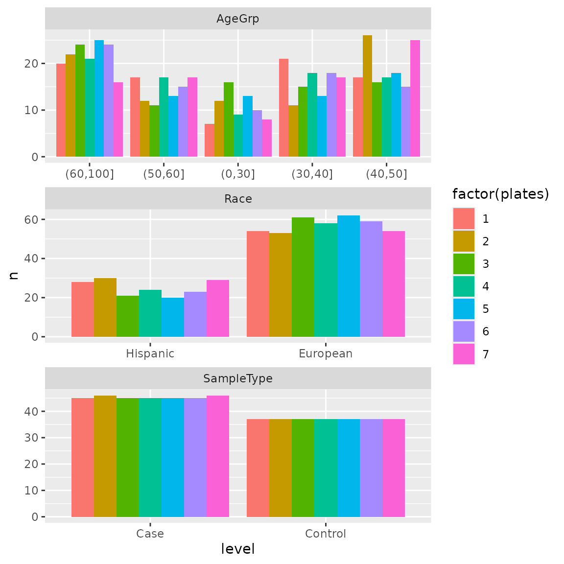
Visualize for plates
plot_batch <- function(df) {
  df |>
    select(plates, SampleType, Race, AgeGrp) |>
    pivot_longer(c(SampleType, Race, AgeGrp), names_to = "variable", values_to = "level") |>
    count(plates, variable, level) |>
    ggplot(aes(level, n, fill = factor(plates))) +
    geom_col(position = "dodge") +
    facet_wrap(~variable, scales = "free", ncol = 1)
}
Before the optimization.
g_setup_start |> plot_batch()
After the optimization.
OSAT::get.experiment.setup(g_setup) |>
  plot_batch()
Compare scores with various implementations
Compare OSAT score generated using designit.
OSAT::getLayout(gc) |>
  left_join(OSAT::get.experiment.setup(g_setup)) |>
  data.table::data.table() |>
  osat_score("plates", c("SampleType", "Race", "AgeGrp")) |>
  with(score)
#> Joining with `by = join_by(plates, chipRows, chipColumns, chips, rows, columns,
#> wells)`
#> Warning in osat_score(data.table::data.table(left_join(OSAT::getLayout(gc), :
#> NAs in features / batch columns; they will be excluded from scoring
#> [1] 34.85714

# score using OSAT
g_setup@metadata$optValue |> tail(1)
#> [1] 34.85714
Run using BatchContainer
First let’s create a BatchContainer with same dimensions.
bc <- BatchContainer$new(
  dimensions = c(plates = 7, chips = 8, rows = 6, columns = 2)
)
bc
#> Batch container with 672 locations.
#>   Dimensions: plates, chips, rows, columns

bc$n_locations
#> [1] 672
Assign samples and get initial setup.
bc <- assign_in_order(bc, samples)

starting_assignment <- bc$get_locations() |>
  left_join(g_setup_start) |>
  pull(ID) |>
  as.integer()
#> Joining with `by = join_by(plates, chips, rows, columns)`

bc$move_samples(location_assignment = starting_assignment)

bc$get_samples(remove_empty_locations = TRUE) |>
  plot_batch()
Using designit OSAT score implementation
scoring_f <- osat_score_generator("plates", c("SampleType", "Race", "AgeGrp"))

bc$score(scoring_f)
#> Warning in osat_score(bc, batch_vars = batch_vars, feature_vars = feature_vars,
#> : NAs in features / batch columns; they will be excluded from scoring
#>  score_1
#> 360.8571
g_setup@metadata$optValue |> head(1)
#> [1] 360.8571
# should be identical

bench::system_time({
  set.seed(123)
  bc_reference <- optimize_design(bc, scoring = scoring_f, max_iter = params$iterations)
})
#> Checking variances of 1-dim. score vector.
#> ... (6749.04) - OK
#> Initial score: 360.857
#> Achieved score: 348.857 at iteration 7
#> Achieved score: 344.857 at iteration 8
#> Achieved score: 338.857 at iteration 10
#> Achieved score: 326.857 at iteration 19
#> Achieved score: 322.857 at iteration 22
#> Achieved score: 320.857 at iteration 24
#> Achieved score: 318.857 at iteration 26
#> Achieved score: 314.857 at iteration 27
#> Achieved score: 308.857 at iteration 28
#> Achieved score: 302.857 at iteration 32
#> Achieved score: 300.857 at iteration 33
#> Achieved score: 292.857 at iteration 36
#> Achieved score: 290.857 at iteration 38
#> Achieved score: 284.857 at iteration 40
#> Achieved score: 276.857 at iteration 45
#> Achieved score: 272.857 at iteration 50
#> Achieved score: 266.857 at iteration 54
#> Achieved score: 258.857 at iteration 55
#> Achieved score: 248.857 at iteration 60
#> Achieved score: 242.857 at iteration 62
#> Achieved score: 224.857 at iteration 71
#> Achieved score: 218.857 at iteration 73
#> Achieved score: 214.857 at iteration 76
#> Achieved score: 204.857 at iteration 78
#> Achieved score: 200.857 at iteration 79
#> Achieved score: 192.857 at iteration 80
#> Achieved score: 184.857 at iteration 84
#> Achieved score: 176.857 at iteration 85
#> Achieved score: 172.857 at iteration 86
#> Achieved score: 170.857 at iteration 95
#> Achieved score: 166.857 at iteration 96
#> Achieved score: 156.857 at iteration 98
#> Achieved score: 150.857 at iteration 99
#> Achieved score: 148.857 at iteration 102
#> Achieved score: 144.857 at iteration 103
#> Achieved score: 138.857 at iteration 113
#> Achieved score: 132.857 at iteration 133
#> Achieved score: 124.857 at iteration 138
#> Achieved score: 120.857 at iteration 140
#> Achieved score: 112.857 at iteration 149
#> Achieved score: 108.857 at iteration 169
#> Achieved score: 106.857 at iteration 175
#> Achieved score: 104.857 at iteration 176
#> Achieved score: 100.857 at iteration 178
#> Achieved score: 98.857 at iteration 179
#> Achieved score: 92.857 at iteration 188
#> Achieved score: 90.857 at iteration 189
#> Achieved score: 86.857 at iteration 190
#> Achieved score: 82.857 at iteration 202
#> Achieved score: 76.857 at iteration 210
#> Achieved score: 72.857 at iteration 223
#> Achieved score: 68.857 at iteration 231
#> Achieved score: 66.857 at iteration 239
#> Achieved score: 64.857 at iteration 262
#> Achieved score: 62.857 at iteration 324
#> Achieved score: 60.857 at iteration 336
#> Achieved score: 58.857 at iteration 358
#> Achieved score: 56.857 at iteration 360
#> Achieved score: 52.857 at iteration 406
#> Achieved score: 50.857 at iteration 419
#> Achieved score: 48.857 at iteration 425
#> Achieved score: 46.857 at iteration 455
#> Achieved score: 42.857 at iteration 505
#> Achieved score: 40.857 at iteration 507
#> Achieved score: 38.857 at iteration 532
#> Achieved score: 36.857 at iteration 618
#> Achieved score: 34.857 at iteration 727
#> Achieved score: 32.857 at iteration 786
#> Achieved score: 30.857 at iteration 960
#> process    real
#>  15.49s   8.03s
# final score
bc_reference$score(scoring_f)
#>  score_1
#> 30.85714
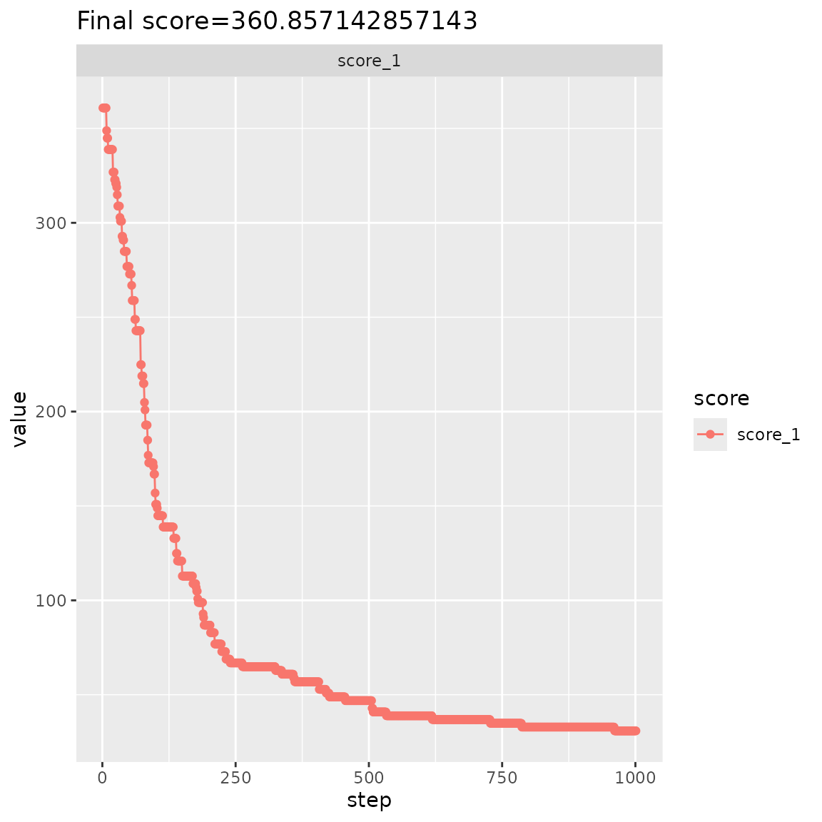
bc_reference$plot_trace() +
  ggtitle(str_glue("Final score={bc$score(scoring_f)}"))
bc$get_samples(remove_empty_locations = TRUE) |>
  plot_batch()
Manually work with data.table
Instead of relying on BatchContainer, here we have a
manual optimization process using data.table.
fast_osat_optimize <- function(bc, batch_vars, feature_vars, iterations) {
  bc <- bc$copy()
  ldf <- data.table::data.table(bc$get_locations())[, c("plates")][, ".sample_id" := bc$assignment]
  fcols <- c(".sample_id", feature_vars)
  smp <- data.table::data.table(bc$samples)[, ..fcols]
  df <- smp[ldf, on = ".sample_id"]

  v <- osat_score(df, batch_vars, feature_vars)
  edf <- v$expected_dt
  current_score <- v$score
  scores <- numeric(length = iterations)
  n_avail <- nrow(df)

  for (i in 1:iterations) {
    repeat {
      pos <- sample(n_avail, 2)

      # does not make sense to shuffle NAs
      if (any(!is.na(df[pos, feature_vars[1]]))) {
        break
      }
    }

    val <- df[c(pos[2], pos[1]), fcols, with = FALSE]
    df[c(pos[1], pos[2]), (fcols) := val]

    new_score <- osat_score(df, batch_vars, feature_vars, edf)$score
    if (new_score <= current_score) {
      current_score <- new_score
    } else {
      df[c(pos[2], pos[1]), (fcols) := val]
    }

    scores[i] <- current_score
  }

  bc$assignment <- df$.sample_id

  list(bc=bc, scores=scores)
}

bench::system_time({
  set.seed(123)
  opt_res <- fast_osat_optimize(bc, "plates", c("SampleType", "Race", "AgeGrp"), iterations = params$iterations)
})
#> Warning in osat_score(df, batch_vars, feature_vars): NAs in features / batch
#> columns; they will be excluded from scoring
#> Warning in (function (assignment) : this field might become read-only in the
#> future, please use $move_samples() instead
#> process    real
#>  10.32s   5.25s
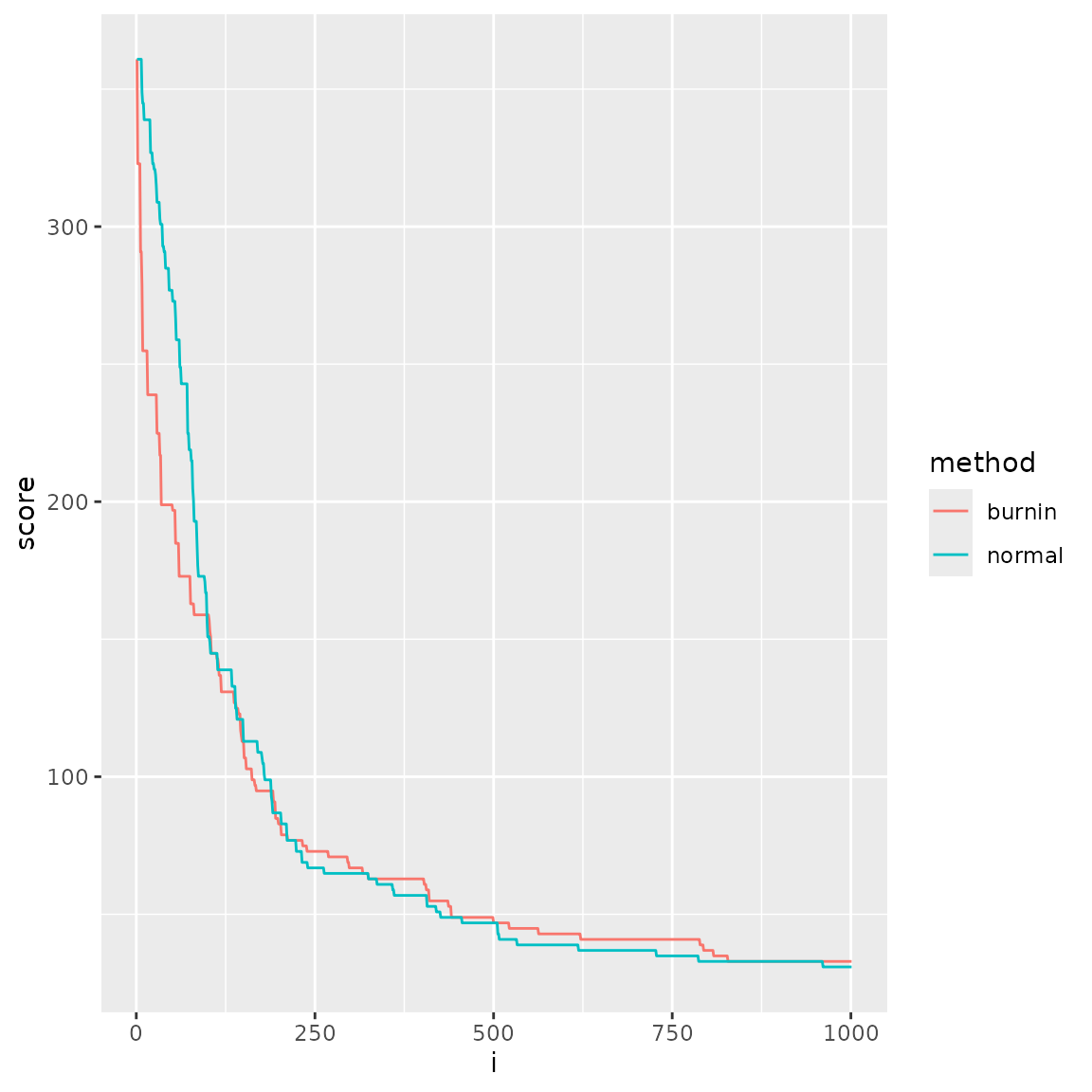
Shuffle optimization with burn-in
scoring_f <- osat_score_generator("plates", c("SampleType", "Race", "AgeGrp"))

burn_in_it <- floor(params$iterations * 0.1)
burn_in_it
#> [1] 100

bench::system_time({
  set.seed(123)
  bc_burn_in <- optimize_design(
    bc,
    scoring = scoring_f,
    n_shuffle = c(
      rep(20, burn_in_it),
      rep(
        2,
        params$iterations - burn_in_it
      )
    ),
    max_iter = params$iterations
  )
})
#> Warning in osat_score(bc, batch_vars = batch_vars, feature_vars = feature_vars,
#> : NAs in features / batch columns; they will be excluded from scoring
#> Checking variances of 1-dim. score vector.
#> ... (5018.697) - OK
#> Initial score: 360.857
#> Achieved score: 322.857 at iteration 1
#> Achieved score: 290.857 at iteration 5
#> Achieved score: 278.857 at iteration 7
#> Achieved score: 254.857 at iteration 8
#> Achieved score: 238.857 at iteration 15
#> Achieved score: 224.857 at iteration 28
#> Achieved score: 216.857 at iteration 32
#> Achieved score: 198.857 at iteration 34
#> Achieved score: 196.857 at iteration 50
#> Achieved score: 184.857 at iteration 54
#> Achieved score: 172.857 at iteration 59
#> Achieved score: 162.857 at iteration 75
#> Achieved score: 158.857 at iteration 80
#> Achieved score: 156.857 at iteration 101
#> Achieved score: 152.857 at iteration 102
#> Achieved score: 150.857 at iteration 103
#> Achieved score: 144.857 at iteration 104
#> Achieved score: 142.857 at iteration 112
#> Achieved score: 140.857 at iteration 114
#> Achieved score: 136.857 at iteration 115
#> Achieved score: 130.857 at iteration 118
#> Achieved score: 126.857 at iteration 136
#> Achieved score: 124.857 at iteration 139
#> Achieved score: 122.857 at iteration 142
#> Achieved score: 116.857 at iteration 145
#> Achieved score: 114.857 at iteration 146
#> Achieved score: 112.857 at iteration 147
#> Achieved score: 106.857 at iteration 150
#> Achieved score: 102.857 at iteration 153
#> Achieved score: 98.857 at iteration 161
#> Achieved score: 96.857 at iteration 165
#> Achieved score: 94.857 at iteration 167
#> Achieved score: 90.857 at iteration 191
#> Achieved score: 84.857 at iteration 194
#> Achieved score: 82.857 at iteration 198
#> Achieved score: 78.857 at iteration 202
#> Achieved score: 76.857 at iteration 211
#> Achieved score: 74.857 at iteration 232
#> Achieved score: 72.857 at iteration 238
#> Achieved score: 70.857 at iteration 268
#> Achieved score: 68.857 at iteration 295
#> Achieved score: 66.857 at iteration 297
#> Achieved score: 64.857 at iteration 316
#> Achieved score: 62.857 at iteration 324
#> Achieved score: 60.857 at iteration 402
#> Achieved score: 58.857 at iteration 405
#> Achieved score: 54.857 at iteration 409
#> Achieved score: 52.857 at iteration 436
#> Achieved score: 48.857 at iteration 440
#> Achieved score: 46.857 at iteration 499
#> Achieved score: 44.857 at iteration 521
#> Achieved score: 42.857 at iteration 562
#> Achieved score: 40.857 at iteration 621
#> Achieved score: 38.857 at iteration 788
#> Achieved score: 36.857 at iteration 793
#> Achieved score: 34.857 at iteration 807
#> Achieved score: 32.857 at iteration 827
#> process    real
#>   15.8s    8.2s
tibble(
  i = bc_burn_in$trace$scores[[1]]$step,
  normal = bc_reference$trace$scores[[1]]$score_1,
  burnin = bc_burn_in$trace$scores[[1]]$score_1
) |>
  pivot_longer(-i, names_to = "method", values_to = "score") |>
  ggplot(aes(i, score, col = method)) +
  geom_line()
Score demonstration
bc$score(scoring_f)
#>  score_1
#> 360.8571
assign_random(bc)
#> Batch container with 672 locations and 576 samples (assigned).
#>   Dimensions: plates, chips, rows, columns

bc$get_samples()
#> # A tibble: 672 × 10
#>    plates chips  rows columns    ID SampleType Race     AgeGrp   dummy_var1
#>     <int> <int> <int>   <int> <dbl> <fct>      <fct>    <fct>         <dbl>
#>  1      1     1     1       1   563 Control    Hispanic (30,40]      0.320
#>  2      1     1     1       2   488 Control    European (30,40]     -1.64
#>  3      1     1     2       1   215 Case       European (50,60]     -1.87
#>  4      1     1     2       2   268 Case       Hispanic (40,50]     -0.639
#>  5      1     1     3       1   165 Case       European (60,100]     0.426
#>  6      1     1     3       2    86 Case       Hispanic (60,100]     0.0756
#>  7      1     1     4       1   264 Case       European (60,100]    -1.45
#>  8      1     1     4       2   451 Control    European (30,40]     -0.827
#>  9      1     1     5       1   250 Case       Hispanic (60,100]     0.405
#> 10      1     1     5       2    NA NA         NA       NA          NA
#> # ℹ 662 more rows
#> # ℹ 1 more variable: dummy_var2 <chr>
bc$get_samples(remove_empty_locations = TRUE)
#> # A tibble: 576 × 10
#>    plates chips  rows columns    ID SampleType Race     AgeGrp   dummy_var1
#>     <int> <int> <int>   <int> <dbl> <fct>      <fct>    <fct>         <dbl>
#>  1      1     1     1       1   563 Control    Hispanic (30,40]      0.320
#>  2      1     1     1       2   488 Control    European (30,40]     -1.64
#>  3      1     1     2       1   215 Case       European (50,60]     -1.87
#>  4      1     1     2       2   268 Case       Hispanic (40,50]     -0.639
#>  5      1     1     3       1   165 Case       European (60,100]     0.426
#>  6      1     1     3       2    86 Case       Hispanic (60,100]     0.0756
#>  7      1     1     4       1   264 Case       European (60,100]    -1.45
#>  8      1     1     4       2   451 Control    European (30,40]     -0.827
#>  9      1     1     5       1   250 Case       Hispanic (60,100]     0.405
#> 10      1     1     6       1   191 Case       Hispanic (60,100]     0.698
#> # ℹ 566 more rows
#> # ℹ 1 more variable: dummy_var2 <chr>

scoring_f <- list(
  fc0 = function(samples) rnorm(1) + 2 * rexp(1),
  fc1 = function(samples) rnorm(1, 100),
  fc2 = function(samples) -7
)

bc$score(scoring_f)
#>       fc0       fc1       fc2
#>   3.64428 100.78084  -7.00000